Signals & Systems — From Time Domain to Spectral Thinking
This note is adapted from course materials for EE3210 Signals and Systems and EE4015 Digital Signal Processing at City University of Hong Kong. Instructors: course teaching staff.
Central Question
Signals and systems theory asks: how does information carried by a time-varying quantity change when it passes through a physical, computational, or communication system?
A signal may be voltage, sound pressure, displacement, packet rate, image intensity, or sensor current. A system is the rule that transforms input into output. The most important tractable class is linear time-invariant systems, because an LTI system is completely described by its impulse response:
\[y(t)=x(t)*h(t), \qquad y[n]=x[n]*h[n].\]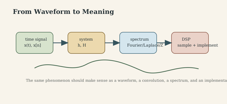
1. Signals: Continuous, Discrete, Energy, and Power
A continuous-time signal $x(t)$ is defined over real time. A discrete-time signal $x[n]$ is defined on integer indices, usually after sampling. Discrete-time is not automatically digital; digital signals also quantize amplitude.
Energy and power separate transient signals from persistent ones:
\[E=\int_{-\infty}^{\infty}|x(t)|^2dt,\] \[P=\lim_{T\to\infty}\frac{1}{2T}\int_{-T}^{T}|x(t)|^2dt.\]A pulse is usually an energy signal. A sinusoid is a power signal. This distinction determines whether Fourier transforms, Fourier series, or generalized functions are the right language.
The impulse $\delta(t)$ is not an ordinary function; it is defined by its sifting action:
\[\int_{-\infty}^{\infty}f(t)\delta(t-t_0)dt=f(t_0).\]That one property explains why an impulse response can characterize an entire LTI system.
2. LTI Systems and Convolution
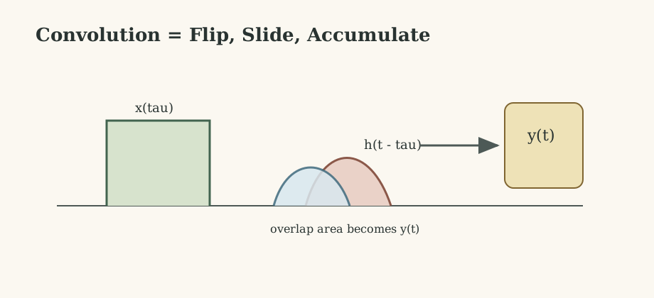
Linearity means superposition. Time invariance means the same input shifted in time produces the same output shifted in time. Together, they imply that an arbitrary input can be decomposed into shifted impulses, each passed through the system, and then summed:
\[y(t)=\int_{-\infty}^{\infty}x(\tau)h(t-\tau)d\tau.\]In discrete time:
\[y[n]=\sum_{k=-\infty}^{\infty}x[k]h[n-k].\]System properties follow from $h$:
- causal if $h(t)=0$ before the input arrives,
-
BIBO stable if $\int h(t) dt<\infty$ or $\sum h[n] <\infty$, - memoryless if $h$ is a scaled impulse,
- invertible if another system $g$ satisfies $h*g=\delta$.
3. Transform Thinking
The deep simplification is that complex exponentials are eigenfunctions of LTI systems. Feeding $e^{st}$ into an LTI system produces the same exponential scaled by $H(s)$.
For continuous time:
\[X(j\omega)=\int_{-\infty}^{\infty}x(t)e^{-j\omega t}dt.\]For discrete time:
\[X(e^{j\Omega})=\sum_{n=-\infty}^{\infty}x[n]e^{-j\Omega n}.\]The decisive property is
\[x*h \quad \Longleftrightarrow \quad XH.\]Hard convolution becomes pointwise multiplication. Filtering becomes spectral shaping.
Laplace and Z transforms extend Fourier analysis by adding convergence regions:
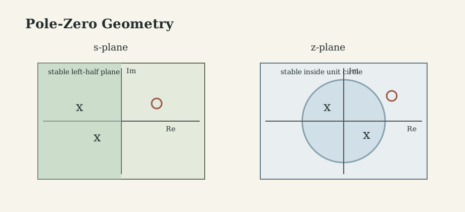
\[H(s)=\frac{Y(s)}{X(s)}, \qquad H(z)=\frac{Y(z)}{X(z)}.\]Poles determine natural modes. Zeros suppress or shape particular components. Continuous-time stability requires poles in the left-half plane; discrete-time stability requires poles inside the unit circle.
4. Sampling and Reconstruction
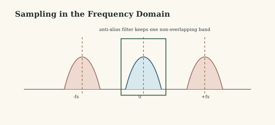
Ideal sampling multiplies a continuous signal by an impulse train. In frequency, this replicates the spectrum at multiples of the sampling frequency. If the replicas overlap, aliasing occurs and lost information cannot be recovered.
The sampling condition is
\[f_s>2f_{\max}.\]This condition is exact only for band-limited signals and ideal filters. Real systems therefore need anti-alias filters, oversampling, aperture/jitter checks, and reconstruction filtering.
Ideal reconstruction uses sinc interpolation:
\[x(t)=\sum_n x[n]\operatorname{sinc}\left(\frac{t-nT_s}{T_s}\right).\]Practical DACs use finite approximations such as zero-order hold plus analog filtering. That implementation introduces droop, delay, and images that must be budgeted in audio, control, communication, and measurement systems.
5. Filters: Analog, FIR, and IIR
Filters are specified by passband, stopband, transition width, ripple, attenuation, group delay, and implementation limits. No physical filter is ideal; all real designs trade selectivity, phase, order, delay, noise, and cost.
Analog filter families express different compromises:
- Butterworth: smooth magnitude, moderate transition,
- Chebyshev: sharper transition with ripple,
- elliptic: sharpest transition with ripple in both bands,
- Bessel: weak selectivity but good time-domain waveform preservation.
Digital filters split into FIR and IIR:
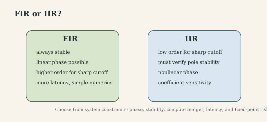
\[y[n]=\sum_{k=0}^{M}b_kx[n-k] \quad \text{(FIR)},\] \[y[n]=\sum_{m=0}^{M}b_mx[n-m]-\sum_{k=1}^{N}a_ky[n-k] \quad \text{(IIR)}.\]FIR filters are always stable and can have exact linear phase with symmetric coefficients, but sharp transitions require many taps. IIR filters achieve sharp responses with low order, but pole placement, coefficient quantization, and nonlinear phase require care.
6. Stochastic Signals and DSP Implementation
Real signals include noise. For a wide-sense stationary process, the autocorrelation and power spectral density form a Fourier pair:
\[S_{XX}(\omega)=\mathcal{F}\{R_{XX}(\tau)\}.\]An LTI system shapes random input spectra by
\[S_{YY}(\omega)=|H(j\omega)|^2S_{XX}(\omega).\]This is the basis of noise filtering, matched filtering, Wiener filtering, and receiver SNR budgeting.
Implementation introduces its own signal transformations: finite word length, overflow, coefficient quantization, sample-clock jitter, latency, and memory layout. A mathematically correct filter can fail in fixed-point arithmetic if scaling and saturation are ignored.
What This Framework Lets Us Do
Signals and systems gives a common language for circuits, control, communications, sensing, audio, imaging, and machine perception. It lets us move between waveform, spectrum, model, and implementation without losing physical meaning.
Where the Framework Stops Being Reliable
The clean theory assumes linearity, time invariance, ideal sampling, exact arithmetic, and known spectra. Saturation, switching, nonlinear sensors, time-varying channels, clock drift, and finite precision require extended models and experiments.
Where the Subject Leads Next
The natural next steps are control theory, communication systems, estimation, stochastic processes, DSP hardware implementation, and machine-learning signal representations.
Technical and Editorial Audit
- Compressed an encyclopedic note into a causal learning path from signals to systems, transforms, sampling, filtering, stochastic analysis, and implementation.
- Preserved the EE3210 and EE4015 course attribution in the main text.
- Added original explanatory figures for the analysis pipeline, convolution, pole-zero stability, sampling, and FIR/IIR tradeoffs.
- Kept standard equations and corrected the emphasis around ideal assumptions versus deployable filters.
- Version-sensitive implementation details such as specific DSP hardware limits should be checked against target datasheets.
Main Sources Used in This Note
- A. V. Oppenheim, A. S. Willsky, and S. H. Nawab, Signals and Systems.
- A. V. Oppenheim and R. W. Schafer, Discrete-Time Signal Processing.
- S. K. Mitra, Digital Signal Processing.
- B. P. Lathi, Linear Systems and Signals.