Data Mining
This note is adapted from course materials for ID2211 Data Mining, Basic Course at KTH Royal Institute of Technology. Instructor: course teaching staff.
Central Question
Data mining asks: how can useful structure be extracted from large, messy data when exact search or exhaustive modeling is too expensive?
The important word is not only data. It is scale. Once data becomes large, algorithm design changes: representation, indexing, sparsity, approximation, streaming, graph structure, and validation become as important as model accuracy.
1. Representation Before Algorithm
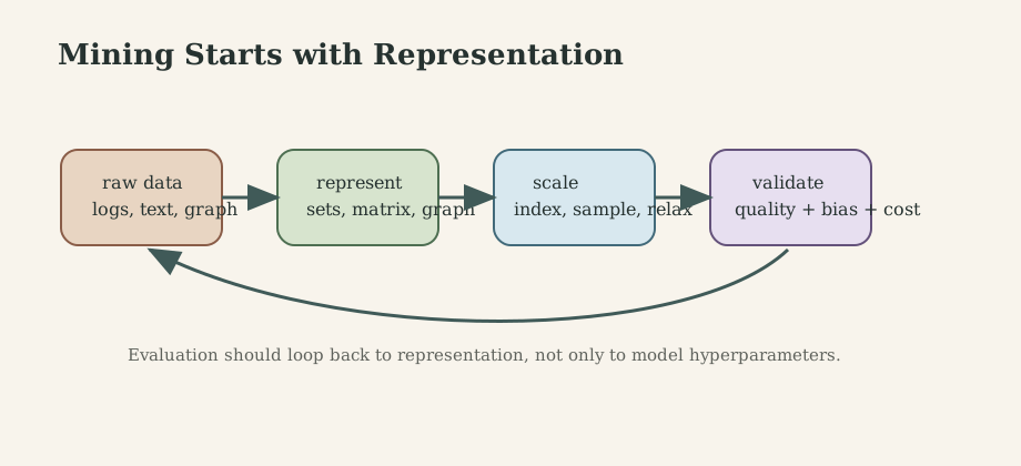
A dataset can be represented as a table, set collection, graph, matrix, text corpus, embedding space, or stream. The same real-world system can support several representations. The choice should follow the task:
- duplicate detection often uses sets and similarity,
- recommendation often uses sparse user-item matrices,
- ranking often uses directed graphs,
- clustering often uses distances or graph cuts,
- prediction often uses features or embeddings.
Poor representation can make a strong algorithm look weak. Good representation can make a simple algorithm surprisingly effective.
2. Similarity Search, MinHash, and LSH
Near-duplicate detection asks for pairs whose distance is small or similarity is high. All-pairs comparison is $O(n^2)$, so scalable systems need candidate generation.
For sets $A$ and $B$, Jaccard similarity is
\[J(A,B)=\frac{|A\cap B|}{|A\cup B|}.\]MinHash gives compact signatures whose collision probability estimates Jaccard similarity. Locality-Sensitive Hashing then places likely-similar items into the same buckets. The workflow is:
- shingle documents or items into sets,
- compute MinHash signatures,
- use LSH bands to generate candidates,
- verify candidates with the exact similarity.
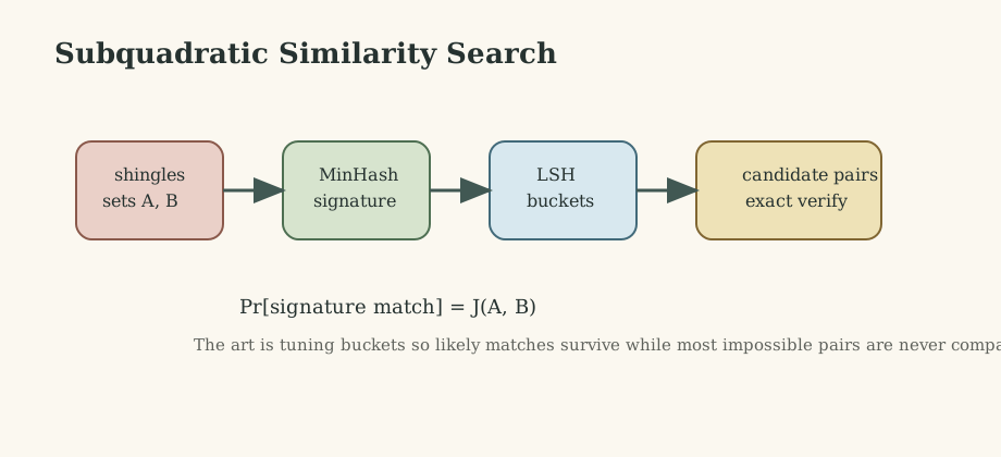
The tuning parameter is not just accuracy. It is the balance between false negatives, false positives, memory, and verification cost.
3. Graph Mining and Link Analysis
Graphs encode relations directly. A graph $G=(V,E)$ can represent webpages, citations, users, roads, dependencies, transactions, or biological interactions.
Basic graph features such as degree, paths, components, clustering coefficient, and local bridges are not decorative. They become inputs to ranking, community detection, anomaly detection, and recommendation.
Random-walk ranking uses a transition matrix $P$:
\[\pi_{t+1}=\pi_tP.\]PageRank adds teleportation:
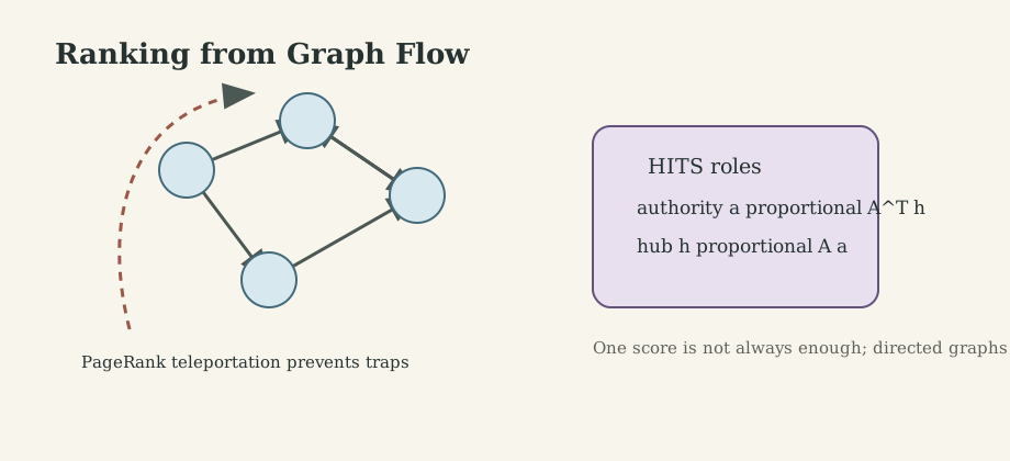
\[\pi=\alpha \pi P+(1-\alpha)v,\]where $v$ is a restart distribution and $\alpha$ controls how much ranking follows links versus teleporting. Teleportation makes the ranking robust to dangling components and disconnected graph structure.
HITS separates two roles:
\[a\propto A^\top h, \qquad h\propto Aa.\]Good authorities are pointed to by good hubs, and good hubs point to good authorities. This role asymmetry is useful in directed information networks.
4. Communities, Cuts, and Spectral Methods
A community is loosely a set of nodes with dense internal connectivity and sparse external connectivity. The difficulty is that this intuition needs an objective.
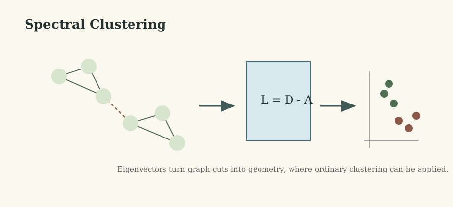
Conductance measures boundary quality relative to volume. Spectral clustering relaxes hard partitioning into linear algebra using the graph Laplacian:
\[L=D-A,\]or the normalized form
\[L_{sym}=I-D^{-1/2}AD^{-1/2}.\]A typical recipe is:
- build a graph or similarity matrix,
- compute informative eigenvectors,
- embed nodes into a low-dimensional spectral space,
- cluster the embedded points.
This converts a combinatorial graph problem into a continuous approximation. It is powerful, but sensitive to graph construction, edge weights, and the selected number of clusters.
5. Low-Rank Models and Recommendation
Large data matrices are often approximately low rank:
\[X\approx U_k\Sigma_kV_k^\top.\]This approximation supports compression, denoising, latent-factor discovery, and recommendation. In a sparse user-item matrix, rows represent users, columns represent items, and latent factors capture hidden preferences or item attributes.
The modeling assumption is not that reality is exactly low-dimensional. It is that the strongest predictive structure can be captured by fewer dimensions than the raw data suggests.
Recommender systems must be evaluated carefully because training data is biased by exposure: users rate items they have already seen or chosen. Good offline metrics should be paired with awareness of popularity bias, cold-start behavior, and feedback loops.
6. Graph Representation Learning
Classical graph mining uses hand-crafted metrics. Representation learning maps nodes, edges, or graphs into vectors:
\[v \mapsto z_v\in\mathbb{R}^k.\]The embedding should preserve a useful notion of proximity: random-walk context, neighborhood similarity, structural role, label information, or task-specific prediction. This unifies matrix factorization, random-walk embeddings, and graph neural models.
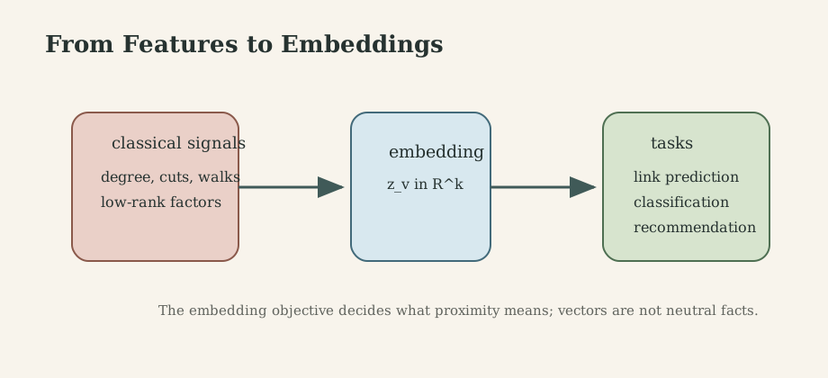
Embeddings are not automatically meaningful. They require negative sampling choices, train-test splits that prevent leakage, baseline comparisons, and interpretation of what proximity actually means.
What This Framework Lets Us Do
Data mining provides scalable methods for similarity search, ranking, clustering, recommendation, anomaly detection, and representation discovery. Its engineering value is in making approximate structure usable under real memory, runtime, and data-quality constraints.
Where the Framework Stops Being Reliable
Data mining can amplify biased samples, leakage, missing-not-at-random behavior, popularity effects, bot activity, and temporal drift. A high score on a static benchmark does not guarantee deployable value if the data-generating process changes.
Where the Subject Leads Next
The natural next steps are machine learning, graph neural networks, information retrieval, recommender-system evaluation, scalable distributed systems, and causal inference.
Technical and Editorial Audit
- Reorganized the original compact notes into representation, similarity search, graph mining, communities, low-rank models, and representation learning.
- Preserved ID2211 course attribution in the body.
- Added original figures for the mining workflow, MinHash/LSH, link analysis, spectral clustering, and representation learning.
- Clarified that approximation quality, runtime, memory, and bias are all part of data-mining evaluation.
- Fast-moving claims about modern graph learning should be verified against current papers before using this as a literature survey.
Main Sources Used in This Note
- J. Leskovec, A. Rajaraman, and J. D. Ullman, Mining of Massive Datasets.
- M. E. J. Newman, Networks.
- C. M. Bishop, Pattern Recognition and Machine Learning.
- Stanford CS224W course materials on graph mining and representation learning.