Data Structures and Algorithms Notes

06 June 2020 - 6 mins read time
Tags: data structures algorithms sorting graph algorithms dynamic programming complexity

This note is adapted from course materials for CS161 Design and Analysis of Algorithms at Stanford University. Instructor: course teaching staff.

Central Question

How do we choose representations and algorithms so that a computation is correct, terminates, and scales under realistic input and memory constraints?

A data structure is a promise about what operations are cheap. An algorithm is a strategy that exploits those promises. The causal spine is:

\[\text{problem specification} \rightarrow \text{representation} \rightarrow \text{invariant} \rightarrow \text{algorithm} \rightarrow \text{correctness proof} \rightarrow \text{complexity} \rightarrow \text{implementation tradeoff}.\]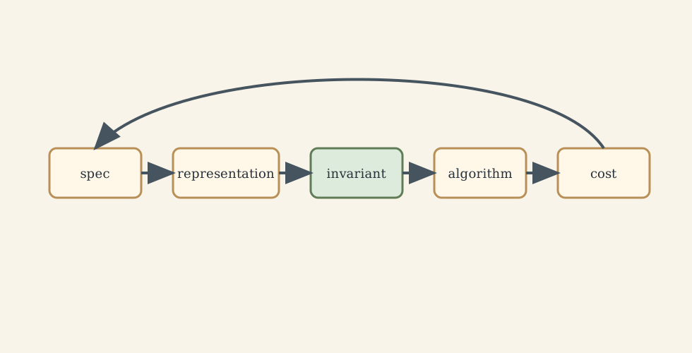

Algorithm design loop from problem specification to representation invariant algorithm correctness complexity and implementation tradeoff — Figure 1. Algorithm design loop. A good algorithm connects specification, representation, invariant, proof, complexity, and implementation cost.

1. Complexity and Correctness

Correctness needs an invariant. For a scan:

maxValue(A):
  best = A[0]
  for each x in A:
    if x > best:
      best = x
  return best

The invariant is: after scanning the first (i) elements, best is the maximum among those elements.

Asymptotic notation describes growth:

(O(f(n))): upper bound;
(\Omega(f(n))): lower bound;
(\Theta(f(n))): tight bound.

Divide-and-conquer often creates recurrences such as

\[T(n)=2T(n/2)+O(n)=\Theta(n\log n).\]

Worst-case analysis is the safest default. Average-case analysis is useful only when the input distribution is justified. Randomization is a design tool when it prevents adversarial structure, as in randomized quicksort.

2. Arrays, Lists, Hash Tables, and Trees

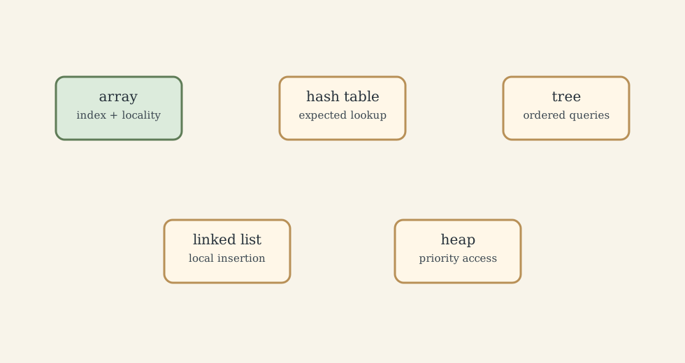
Representation controls cost.

Data structure cost map comparing arrays linked lists hash tables trees heaps and graphs — Figure 2. Representation cost map. Arrays buy indexing and locality; linked structures buy cheap local insertion; hash tables buy expected lookup; trees buy order.

Structure	Cheap operation	Expensive or fragile operation
Array / dynamic array	indexing, scan, cache-friendly iteration	middle insertion/deletion
Linked list	insertion when node is known	search and cache locality
Stack	last-in-first-out push/pop	arbitrary access
Queue	first-in-first-out enqueue/dequeue	arbitrary access
Hash table	expected lookup/insert/delete	worst-case collisions, resizing
Balanced tree	ordered lookup/range queries	pointer overhead, rotations
Heap	min/max priority access	arbitrary search

Binary search is (O(\log n)) only because sorted arrays provide cheap random access. A linked list can be sorted but cannot support efficient binary search because “middle” is not cheap.

3. Sorting and Lower Bounds

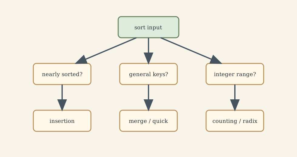
Sorting algorithms are best read as invariant patterns:

insertion sort maintains a sorted prefix;
selection sort grows a prefix of globally selected minima;
merge sort recursively sorts and merges;
quicksort partitions around a pivot;
counting/radix sort exploit key structure rather than comparisons.

Comparison sorting has an (\Omega(n\log n)) lower bound because the algorithm must distinguish among (n!) possible orderings. Counting and radix sort can beat this only by assuming more about keys.

Sorting decision tree comparing insertion merge quick counting and radix sort by input size order and key assumptions — Figure 3. Sorting decision logic. Comparison sorts are general; counting and radix sorts are faster only when key assumptions are available.

Algorithm	Time	Strength	Main condition
Insertion sort	(O(n^2)) worst	simple, good on nearly sorted data	small or nearly sorted input
Merge sort	(O(n\log n))	predictable, stable	extra memory acceptable
Quicksort	(O(n\log n)) average	fast in-memory	pivot strategy matters
Counting sort	(O(n+k))	linear-like	small integer key range
Radix sort	(O(d(n+k)))	avoids comparisons	digit/key representation known

4. Graphs: Structure Before Algorithm

A graph is (G=(V,E)). Representation changes cost:

adjacency list: efficient for sparse graphs;
adjacency matrix: efficient edge queries and dense graphs;
edge list: useful for Kruskal-style processing.

Traversal algorithms expose reachability:

BFS explores by layers and gives shortest paths in unweighted graphs;
DFS explores depth and reveals cycles, topological order, and components.

Shortest paths depend on assumptions:

BFS: unweighted edges;
Dijkstra: nonnegative edge weights;
Bellman-Ford: negative edges allowed, detects negative cycles;
Floyd-Warshall: all-pairs dynamic programming.

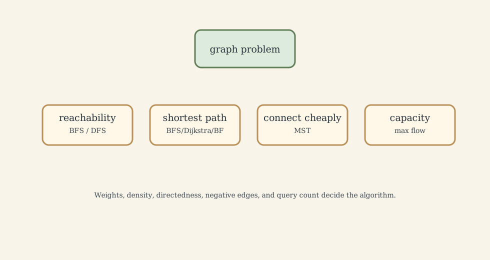
Graph algorithm selection map for BFS DFS Dijkstra Bellman Ford MST and flow — Figure 4. Graph algorithm choice depends on graph representation, edge weights, density, and the query being asked.

Minimum spanning trees solve a different problem: connect all vertices with minimum total edge cost, not shortest paths from a source. Kruskal sorts edges and uses disjoint sets; Prim grows a tree from a frontier.

Flow algorithms model capacity-constrained movement. They are useful when “how much can pass through the network?” is the real question.

5. Dynamic Programming and Greedy Algorithms

Dynamic programming works when a problem has overlapping subproblems and optimal substructure. The method is:

define the state;
define the recurrence;
set base cases;
choose evaluation order;
recover the solution if needed.

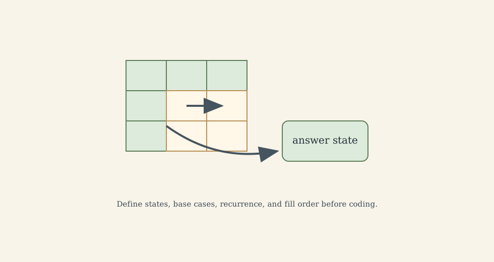
Dynamic programming state transition graph showing base cases recurrence table fill order and answer extraction — Figure 5. Dynamic programming turns repeated recursion into a state table with explicit transitions and base cases.

Memoization starts from recursion and caches results. Tabulation starts from dependencies and fills a table. Both are the same recurrence with different execution orders.

Greedy algorithms make locally optimal choices. They are correct only when an exchange argument, cut property, matroid structure, or monotonic invariant proves that the local choice can be part of a global optimum. Dijkstra, Kruskal, and interval scheduling are not correct because they “feel intuitive”; they are correct because their choices satisfy structural conditions.

6. Choosing the Right Tool

Good DSA practice asks:

what operation dominates?
is the input sorted, weighted, dense, sparse, static, or streaming?
do we need exactness or approximation?
is worst-case behavior important?
is memory locality more important than asymptotic notation?
can preprocessing make many later queries cheap?

The best algorithm is rarely the fanciest. It is the one whose assumptions match the problem and whose invariant is simple enough to trust.

What This Framework Lets Us Do

It lets us move from “memorize algorithms” to “select mechanisms”: arrays for locality, heaps for priority, hash tables for expected lookup, trees for order, BFS for layers, Dijkstra for nonnegative weighted paths, DP for overlapping states, greedy when local choices are provably safe.

Where the Framework Stops Being Reliable

Asymptotics can hide constants, memory locality, cache misses, allocation overhead, adversarial inputs, recursion depth, numerical precision, and distributed-system costs. Implementation evidence still matters.

Where the Subject Leads Next

DSA leads to compilers, databases, operating systems, machine learning systems, distributed systems, graph mining, optimization, and parallel algorithms.

Technical and Editorial Audit

Area	Correction or decision
Central question	Reframed DSA around representation, invariants, proof, and scaling.
Preserved material	Kept arrays, lists, sorting, hashing, trees, graphs, shortest paths, MST, flow, DP, greedy, and complexity.
Figures	Added five original SVG diagrams for algorithm design, representation costs, sorting choice, graph choice, and DP transitions.
Main correction	Emphasized assumptions behind each algorithm rather than presenting algorithms as standalone recipes.

Main Sources Used in This Note

Stanford CS161 course material.