Materials Engineering Notes - Structure, Properties, Processing, and Failure
This note is adapted from course materials for MNE2110 Engineering Materials at City University of Hong Kong. Instructor: course teaching staff.
Central Question
How do atomic bonding, structure, defects, processing history, and environment determine what a material can safely do in an engineering system?
Materials science exists because “steel,” “silicon,” “polymer,” or “ceramic” is never the whole answer. The same chemistry can be soft or hard, ductile or brittle, conductive or insulating, corrosion-resistant or vulnerable, depending on processing and structure. A component fails not because a material name failed, but because a structure-property-environment combination reached its limit.
The central loop is:
\[\text{processing} \rightarrow \text{structure} \rightarrow \text{properties} \rightarrow \text{performance} \rightarrow \text{failure feedback}.\]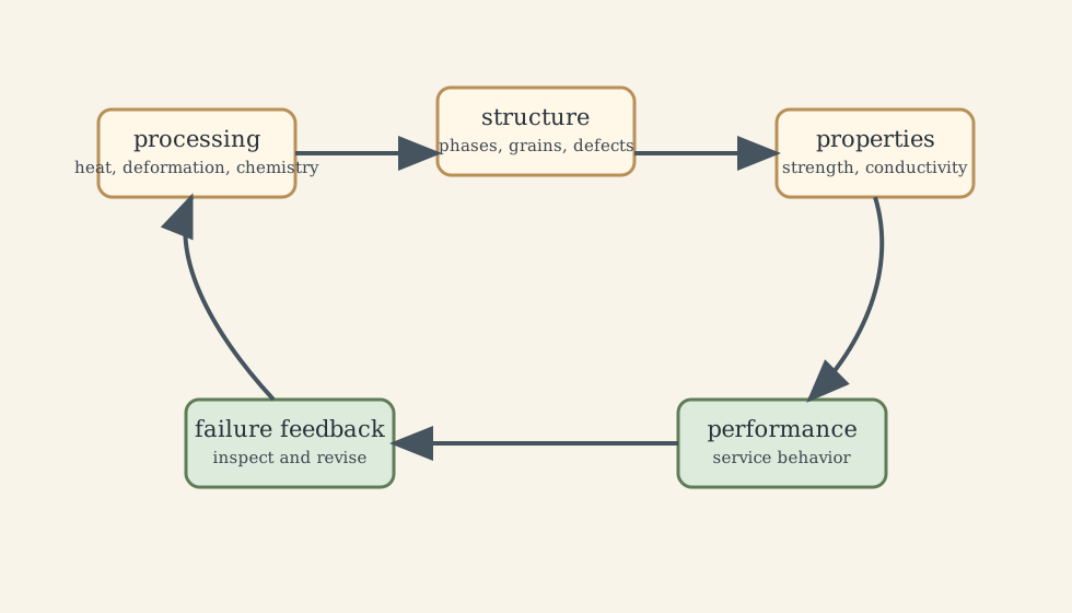
1. Bonding: Why Material Families Behave Differently
Bonding sets the first boundary conditions for material behavior:
- metallic bonding has delocalized electrons, giving electrical and thermal conductivity plus ductility because bonds can rearrange during slip;
- ionic bonding gives strong electrostatic attraction but often brittle fracture when like charges are forced together by shear;
- covalent bonding is directional, producing high stiffness and high temperature capability in networks such as diamond, silicon carbide, and silicon;
- secondary bonding controls polymer chain mobility, molecular crystals, water, biological molecules, and many soft materials.
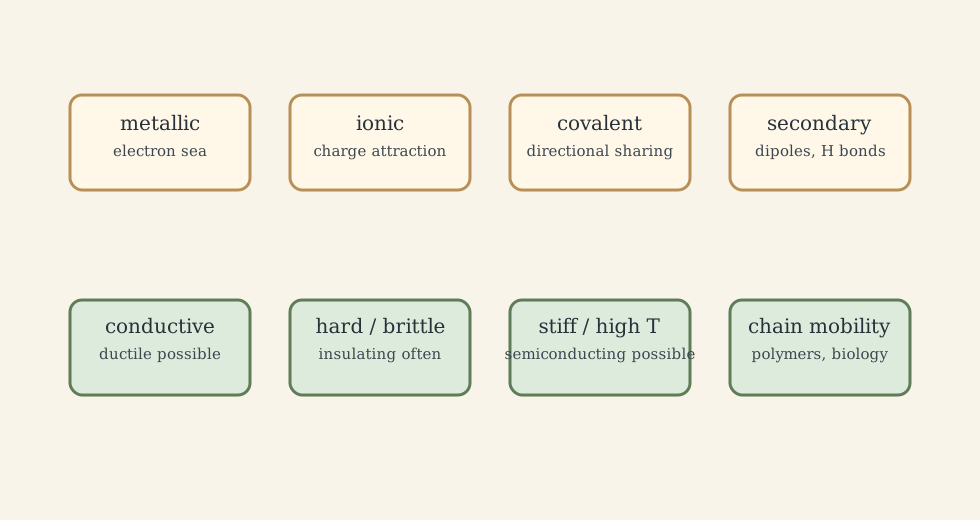
Bonding does not determine everything, but it defines what is plausible. Alloying can greatly change strength, corrosion resistance, and phase stability, yet Young’s modulus for a metal family usually changes far less than yield strength because modulus is tied strongly to bond stiffness.
2. Crystal Structure and Slip
Most engineering metals are crystalline. Crystal structure matters because plastic deformation occurs mainly by dislocation slip on specific planes and directions.
2.1 FCC, BCC, and HCP
FCC metals such as Al, Cu, Ni, Au, and austenitic stainless steel have close-packed ({111}) planes and many slip systems. They are usually ductile because dislocations have multiple easy paths.
BCC metals such as ferrite, Cr, Mo, and W do not have true close-packed planes. Screw dislocation motion can be temperature-sensitive, so many BCC alloys show ductile-to-brittle transition behavior.
HCP metals such as Mg, (\alpha)-Ti, Zn, and Zr have fewer easy slip systems at room temperature. Additional prismatic or pyramidal slip often needs higher stress or temperature, which is why many HCP alloys are harder to cold-form.
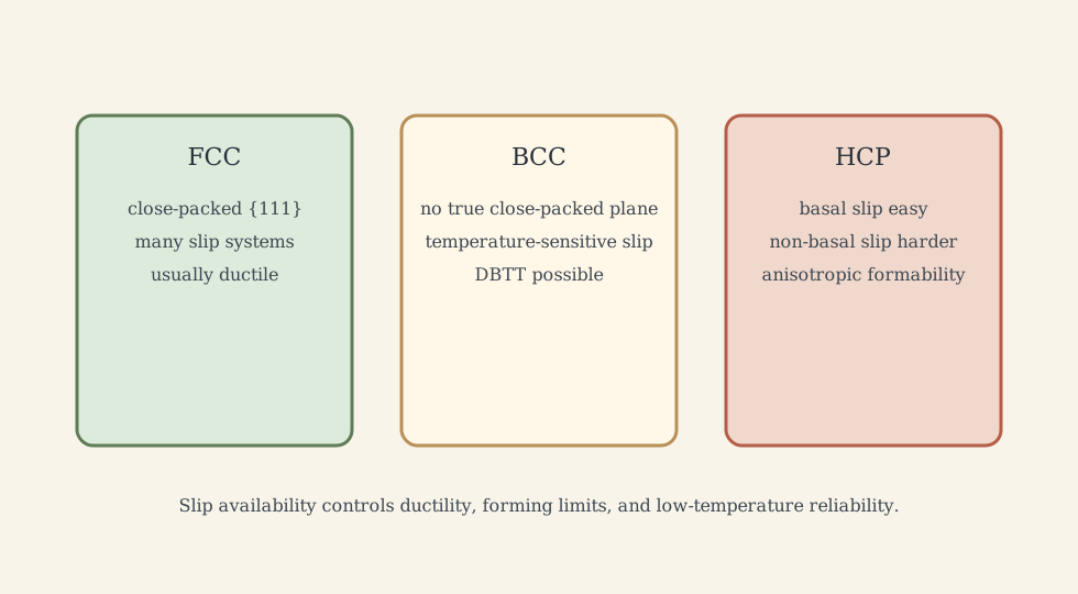
The engineering consequence is immediate: formability, toughness, anisotropy, and low-temperature reliability depend on crystal structure as well as composition.
2.2 Defects Are Functional, Not Just Imperfections
Perfect crystals are mostly a teaching device. Real properties come from defects:
- vacancies enable substitutional diffusion;
- interstitials such as C and N strongly distort metals;
- dislocations enable plastic deformation at realistic stresses;
- grain boundaries impede slip and support diffusion/corrosion paths;
- stacking faults and twins change work hardening and deformation modes;
- precipitates and inclusions can strengthen, embrittle, or initiate cracks.
The vacancy concentration follows an activated form:
\[n_v = N \exp\left(-\frac{Q_v}{k_B T}\right),\]where (n_v) is vacancy count, (N) is available lattice sites, (Q_v) is vacancy formation energy, (k_B) is Boltzmann’s constant, and (T) is absolute temperature.
3. Strengthening: Make Dislocations Harder to Move
Plastic deformation in crystalline metals occurs because dislocations move. Strengthening mechanisms work by obstructing that motion.
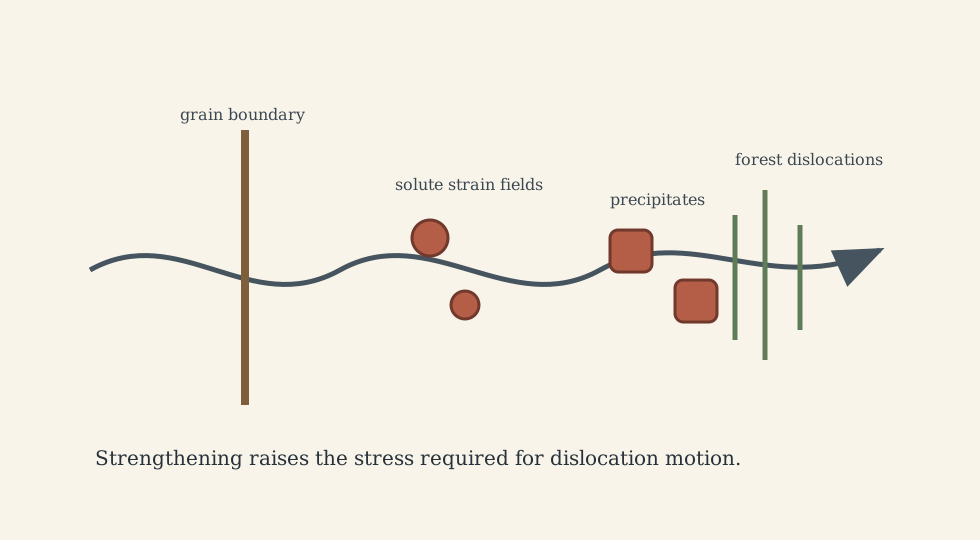
Important mechanisms:
- grain refinement: grain boundaries block pile-ups, often summarized by Hall-Petch;
- solid solution strengthening: solute atoms create strain fields that interact with dislocations;
- precipitation hardening: particles are cut or bypassed by dislocations;
- work hardening: deformation increases dislocation density and forest interactions;
- transformation strengthening: phase changes such as martensite formation or TRIP absorb energy and raise strength.
The Hall-Petch relation is
\[\sigma_y = \sigma_0 + k d^{-1/2},\]where (\sigma_y) is yield strength, (\sigma_0) is lattice/friction stress, (k) is a material constant, and (d) is grain diameter. It is a useful engineering trend, not a universal law down to arbitrarily small grains.
Precipitation hardening has an optimum aging window. Under-aging produces too few or too small obstacles. Peak aging gives strong obstruction. Over-aging coarsens precipitates and increases spacing, reducing strength.
4. Phase Diagrams, Diffusion, and Heat Treatment
Thermodynamics tells us which phases are stable; kinetics tells us how fast transformations occur.
The Gibbs free energy relation is
\[G = H - TS,\]where (G) is Gibbs free energy, (H) is enthalpy, (T) is absolute temperature, and (S) is entropy. Phase diagrams map equilibrium phase stability versus temperature and composition.
Diffusion obeys Fick-type laws:
\[J = -D\frac{dC}{dx}, \qquad \frac{\partial C}{\partial t}=D\frac{\partial^2 C}{\partial x^2},\]with an Arrhenius diffusion coefficient:
\[D = D_0 \exp\left(-\frac{Q}{RT}\right).\]This exponential temperature dependence is why heat treatment works: a small temperature change can strongly change diffusion rate and transformation time.
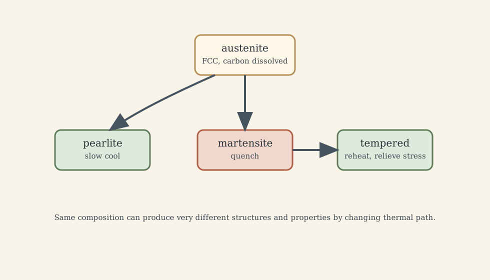
For steels, the iron-carbon diagram is the central map:
- austenite ((\gamma)): FCC phase with higher carbon solubility;
- ferrite ((\alpha)): BCC phase with low carbon solubility;
- cementite (\mathrm{Fe_3C}): hard brittle carbide;
- pearlite: ferrite-cementite lamellae from slow cooling near eutectoid conditions;
- martensite: diffusionless supersaturated body-centered tetragonal structure formed by quenching;
- tempered martensite: martensite reheated to reduce brittleness while retaining strength.
The lever rule in a two-phase region is a mass balance:
\[W_\alpha = \frac{C_0-C_\beta}{C_\alpha-C_\beta}, \qquad W_\beta = \frac{C_\alpha-C_0}{C_\alpha-C_\beta}.\]Use it only inside a two-phase equilibrium region with compositions read from the tie line.
5. Mechanical Behavior, Fracture, and Fatigue
Elastic deformation is reversible:
\[\sigma = E\varepsilon,\]where (\sigma) is stress, (E) is Young’s modulus, and (\varepsilon) is strain. Plastic deformation begins when dislocations move irreversibly.
Fracture begins with flaws. For mode-I cracks,
\[K_I = Y\sigma\sqrt{\pi a},\]where (K_I) is stress intensity, (Y) is a geometry factor, (\sigma) is nominal stress, and (a) is crack size. Fast fracture occurs when (K_I\ge K_{IC}), where (K_{IC}) is fracture toughness.
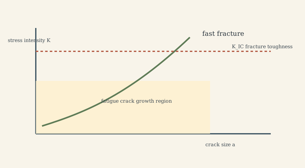
Fatigue can grow cracks below (K_{IC}). A common crack-growth model is Paris’ law:
\[\frac{da}{dN}=C(\Delta K)^m,\]where (a) is crack length, (N) is load cycles, (\Delta K) is stress-intensity range, and (C,m) are material/environment constants. This is why inspection intervals matter: the engineering question is how long an undetected crack takes to grow to critical size.
Ceramics fail differently because crack-tip plasticity is limited. Weibull statistics are often needed because strength depends on flaw population and stressed volume. Larger ceramic parts tend to be weaker statistically because they are more likely to contain a critical flaw.
6. Semiconductors, Doping, and Functional Materials
Band structure controls electrical behavior:
- metals have available electronic states at the Fermi level;
- semiconductors have a moderate bandgap;
- insulators have a large bandgap.
Conductivity is approximately
\[\sigma = nq\mu_e + pq\mu_h,\]where (n,p) are electron and hole concentrations, (q) is elementary charge, and (\mu_e,\mu_h) are mobilities.
Doping silicon with donor atoms creates n-type material; acceptor atoms create p-type material. A p-n junction forms a depletion region and built-in electric field. This is the mechanism behind diodes, solar cells, LEDs, and transistor junctions.
Mobility is limited by phonon scattering, impurity scattering, and microstructure. Higher doping increases carriers but can reduce mobility. This is a typical materials tradeoff: improving one factor can degrade another.
7. Polymers, Ceramics, Glasses, Coatings, and Corrosion
7.1 Polymers
Polymers are governed by chain mobility. Below the glass transition temperature (T_g), chain segments are frozen and the polymer is glassy. Above (T_g), segmental motion increases and the response becomes rubbery or flow-like depending on architecture.
Linear and branched thermoplastics can soften and flow; crosslinked thermosets cannot melt without degradation. Viscoelasticity means response depends on time scale: fast loading may look stiff, while long loading causes creep or stress relaxation.
7.2 Ceramics and Glasses
Ceramics have high stiffness, hardness, melting point, and chemical stability because of strong ionic/covalent bonding. They are brittle because dislocation motion and crack-tip plasticity are limited at ordinary temperatures.
Glass is metastable. Annealing reduces residual stress; tempering creates beneficial surface compression; chemical strengthening uses ion exchange to create compressive surface layers.
7.3 Surfaces and Coatings
Surfaces are chemically and mechanically different from bulk material. PVD, CVD, ALD, electroplating, nitriding, carburizing, shot peening, and thermal spray all modify surface function. The purpose may be wear resistance, corrosion protection, fatigue improvement, thermal insulation, optical response, or electronic function.
7.4 Corrosion
Corrosion is an electrochemical cell:
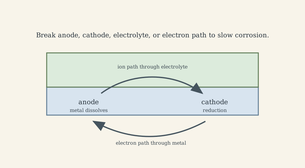
- anode: metal oxidation, such as (\mathrm{Fe\rightarrow Fe^{2+}+2e^-});
- cathode: reduction reaction consuming electrons;
- electrolyte: ion path;
- metallic path: electron path.
Protection strategies include material selection, passivation, coatings, cathodic protection, drainage, crevice avoidance, galvanic isolation, and residual tensile-stress reduction.
8. Composites and Biomaterials
Composites combine phases so that architecture carries load. For continuous aligned fibers loaded parallel to the fibers,
\[E_1 = V_fE_f + V_mE_m,\]an isostrain rule of mixtures. Perpendicular stiffness is closer to an isostress bound:
\[\frac{1}{E_2}=\frac{V_f}{E_f}+\frac{V_m}{E_m}.\]This anisotropy is the power and danger of composites. A laminate must be designed for actual load paths, impact damage, delamination, moisture, inspection, and repair.
Biomaterials add a biological boundary condition. Biocompatibility is not a standalone material property; it depends on material, surface, geometry, mechanical load, degradation, sterilization, and the tissue environment. Titanium can be successful as an implant surface and unacceptable as free ions in blood. Bone, tendon, cartilage, and skin are hierarchical composites, which is why replacing them is harder than matching one number such as modulus.
9. Material Selection and Characterization
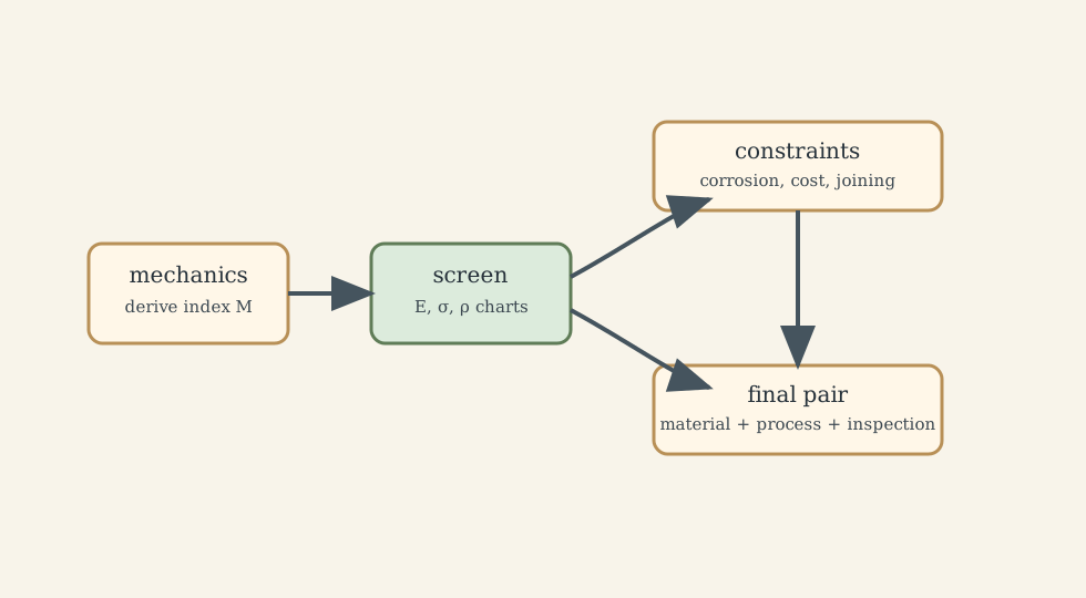
Material selection is constrained optimization. Ashby-style performance indices connect structural mechanics to material charts. For example, a light stiff beam may use an index like
\[M=\frac{E^{1/3}}{\rho},\]while a light strong panel may involve (\sigma_y^{1/2}/\rho). The index screens candidates, but final selection must add corrosion, processing, joining, cost, supply, sustainability, safety, and inspection constraints.
Characterization closes the loop:
- XRD identifies phases and texture;
- SEM/EDS reveals morphology, fracture surfaces, and chemistry;
- TEM reveals dislocations, precipitates, and interfaces;
- EBSD maps grain orientation and texture;
- tensile tests measure modulus, yield, UTS, ductility;
- hardness provides fast local property screening;
- fracture toughness and fatigue tests quantify damage tolerance;
- nanoindentation supports thin films and small volumes.
The key is to match the test to the failure mechanism. Measuring hardness does not prove fatigue resistance; measuring tensile strength does not prove corrosion resistance.
What This Framework Lets Us Do
This framework lets us reason from mechanism to design:
- bonding limits broad material-family behavior;
- crystal structure and defects explain plasticity;
- processing changes microstructure;
- microstructure changes strength, toughness, conductivity, corrosion, and fatigue;
- environment and loading determine which failure mode dominates;
- characterization tests whether the assumed structure actually exists.
Where the Framework Stops Being Reliable
The framework becomes unreliable when a material is treated as a database row. Real properties depend on supplier route, heat treatment, geometry, surface condition, residual stress, manufacturing defects, environment, and inspection history. Numbers in handbooks are starting assumptions, not guarantees.
Where the Subject Leads Next
Materials connects directly to manufacturing, mechanics, electronics, microfabrication, biomaterials, failure analysis, sustainability, and design optimization. The practical skill is to choose a material-process-inspection combination, not merely a material name.
Technical and Editorial Audit
| Area | Correction or decision |
|---|---|
| Central question | Reframed materials as processing-structure-property-performance-failure reasoning. |
| Preserved material | Retained bonding, FCC/BCC/HCP, defects, doping, mechanical behavior, phase diagrams, diffusion, polymers, ceramics, coatings, corrosion, composites, biomaterials, selection, and characterization. |
| Equations | Kept vacancy concentration, Hall-Petch, Gibbs free energy, Fick’s laws, Arrhenius diffusion, lever rule, Hooke’s law, stress intensity, Paris law, conductivity, rule of mixtures, and selection indices. |
| Units and assumptions | Clarified key symbols and where models are trends, bounds, or mechanism-specific relations. |
| Figures | Added eight original SVG diagrams for the PSP loop, bonding map, crystal slip, strengthening, heat treatment, fracture/fatigue, corrosion cell, and selection logic. |
| Editorial correction | Reduced anecdotal over-certainty and shifted examples into mechanism-based explanations. |
Main Sources Used in This Note
- CityU MNE2110 course material.
- Standard materials-science references such as Callister and Rethwisch, Materials Science and Engineering.