Numerical Linear Algebra and Optimization Notes
This note is a personal synthesis of numerical linear algebra, scientific computing, and optimization references. I have not attached a specific university course code to this version because the source notes did not identify one.
Central Question
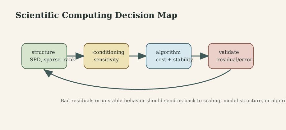
Numerical linear algebra and optimization ask: how do we compute reliable answers when exact algebra is too expensive, data is noisy, and floating-point arithmetic is imperfect?
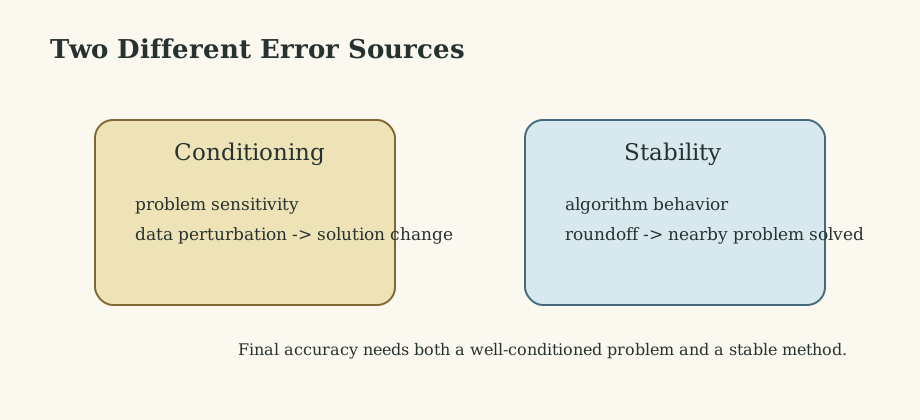
The core distinction is between the mathematical problem and the algorithm used to solve it. A problem can be ill-conditioned even if the algorithm is stable; an algorithm can be unstable even for a well-conditioned problem.
1. Conditioning, Stability, and Floating Point
Floating-point arithmetic is modeled as
\[\operatorname{fl}(a\circ b)=(a\circ b)(1+\delta), \qquad |\delta|\le u,\]where $u$ is machine precision. This model is simple, but it explains why algorithmic rearrangement changes numerical behavior.
Conditioning measures problem sensitivity. For a nonsingular linear system,
\[\kappa_2(A)=\|A\|_2\|A^{-1}\|_2=\frac{\sigma_{\max}}{\sigma_{\min}}.\]A perturbation estimate is
\[\frac{\|\Delta x\|}{\|x\|} \lesssim \kappa(A)\left(\frac{\|\Delta A\|}{\|A\|}+\frac{\|\Delta b\|}{\|b\|}\right).\]Stability measures whether the algorithm solves a nearby problem. Backward stability is especially valuable because it says the computed answer is exact for slightly perturbed input data.
2. Direct Linear Solvers
Dense Gaussian elimination factors a matrix into triangular pieces:
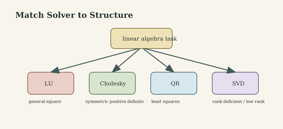
\[PA=LU.\]The factorization costs about $\frac{2}{3}n^3$ operations for dense matrices, with triangular solves costing $O(n^2)$ per right-hand side. Pivoting controls small pivots and roundoff growth.
For symmetric positive definite matrices, Cholesky is preferred:
\[A=LL^\top.\]It is cheaper than LU and backward stable for SPD problems.
QR factorization is the workhorse for orthogonality-sensitive problems:
\[A=QR.\]Householder QR is usually the dense default because it preserves orthogonality better than classical Gram-Schmidt.
3. Least Squares, Rank Deficiency, and SVD
Least squares solves
\[\min_x\|Ax-b\|_2.\]The normal equations
\[A^\top Ax=A^\top b\]are compact but can square the condition number:
\[\kappa(A^\top A)=\kappa(A)^2.\]QR avoids that amplification for many problems. When rank deficiency or near-dependence matters, the singular value decomposition is safer:
\[A=U\Sigma V^\top, \qquad A^+=V\Sigma^+U^\top.\]The SVD also gives the best rank-$k$ approximation:
\[\|A-A_k\|_2=\sigma_{k+1}.\]This is the linear algebra foundation of compression, denoising, principal components, and low-rank modeling.
4. Eigenvalues and Iterative Linear Solvers
Eigenvalue algorithms expose modes:
\[Ax=\lambda x.\]Power iteration converges to the dominant eigenvector when the starting vector has a component in that direction:
\[x_{k+1}=\frac{Ax_k}{\|Ax_k\|}.\]| The rate depends on the spectral gap, roughly $ | \lambda_2/\lambda_1 | $. QR algorithms and Krylov methods generalize this idea into practical eigenvalue computation. |
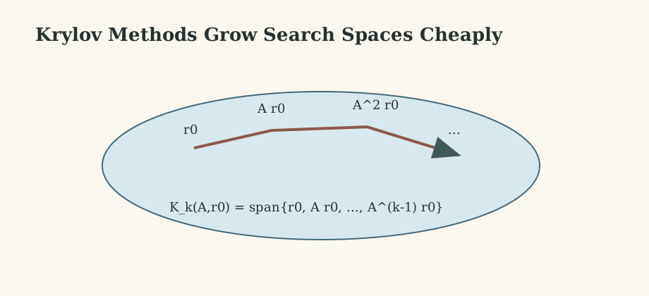
For large sparse systems, storing and factoring $A$ may be impossible. Iterative methods use matrix-vector products and subspaces:
\[\mathcal{K}_k(A,r_0)=\operatorname{span}\{r_0,Ar_0,\ldots,A^{k-1}r_0\}.\]Conjugate Gradient solves SPD systems by minimizing the quadratic energy. Its convergence is bounded by
\[\frac{\|e_k\|_A}{\|e_0\|_A} \le 2\left(\frac{\sqrt{\kappa}-1}{\sqrt{\kappa}+1}\right)^k.\]GMRES handles general nonsymmetric systems by minimizing residuals over Krylov subspaces, but memory and orthogonalization cost grow unless restarted.
5. Optimization: Geometry of Descent
Unconstrained optimization solves
\[\min_x f(x).\]Gradient descent uses local slope:
\[x_{k+1}=x_k-\alpha_k\nabla f(x_k).\]For smooth convex objectives with suitable step size, the method converges sublinearly; strong convexity gives linear convergence. Newton’s method uses a quadratic local model:
\[m_k(p)=f_k+\nabla f_k^\top p+\frac{1}{2}p^\top\nabla^2f_kp.\]It can converge quadratically near a solution but needs globalization such as line search or trust regions. Quasi-Newton methods such as BFGS approximate curvature from gradient differences:
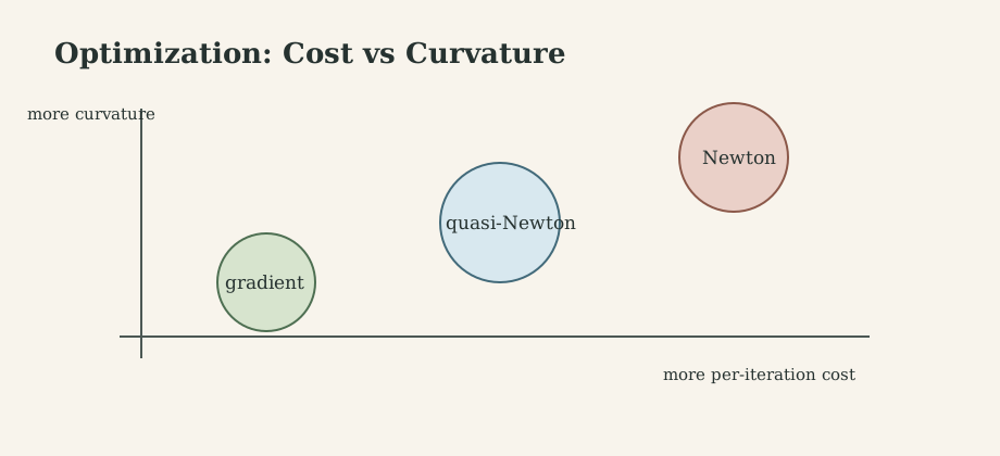
\[B_{k+1}s_k=y_k.\]The practical hierarchy is: gradient methods are cheap but may be slow; Newton methods are fast near a solution but expensive; quasi-Newton methods often give a strong engineering compromise.
6. Constraints, Sparsity, and Scale
Constrained problems introduce feasibility:
\[\min_x f(x)\quad\text{s.t.}\quad g(x)\le0,\; h(x)=0.\]Karush-Kuhn-Tucker conditions combine stationarity, feasibility, complementary slackness, and regularity assumptions. Quadratic programs, interior-point methods, augmented Lagrangians, and ADMM are different ways to manage these conditions.
Large-scale computing changes the priority order. Memory movement, sparsity pattern, preconditioning, communication cost, and parallelism may dominate arithmetic counts. Sparse storage formats such as CSR and CSC matter because they preserve structure and avoid dense $O(n^3)$ bottlenecks.
Stochastic optimization uses noisy gradients:
\[x_{k+1}=x_k-\alpha_kg_k,\qquad \mathbb{E}[g_k]=\nabla f(x_k).\]The central trade is cheaper updates versus variance. Variance reduction, minibatching, adaptive preconditioning, and distributed consensus methods all address this trade from different angles.
What This Framework Lets Us Do
This subject gives the computational backbone for simulation, data fitting, machine learning, control, inverse problems, and scientific modeling. It teaches how to choose algorithms based on structure, error, memory, and convergence evidence.
Where the Framework Stops Being Reliable
Theorems usually assume exact structure: SPD matrices, Lipschitz gradients, convexity, independent samples, or exact arithmetic models. Real problems may violate these assumptions through scaling, bad units, missing data, nonsmooth objectives, or hardware limits.
Where the Subject Leads Next
The next steps are sparse direct solvers, preconditioning, randomized numerical linear algebra, convex optimization, automatic differentiation, scientific machine learning, and distributed optimization.
Technical and Editorial Audit
- Compressed a full syllabus-style reference into a decision-oriented scientific-computing note.
- Marked the attribution as personal synthesis because no source course code was present in the file.
- Added original figures for numerical decision flow, conditioning versus stability, direct solver selection, Krylov subspaces, and optimization tradeoffs.
- Preserved central equations for floating point, condition number, LU/Cholesky/QR, least squares, SVD, Krylov methods, CG, gradient descent, Newton, constraints, and SGD.
- Detailed convergence constants and implementation choices should be verified for the specific matrix class or optimization assumptions.
Main Sources Used in This Note
- L. N. Trefethen and D. Bau III, Numerical Linear Algebra.
- G. H. Golub and C. F. Van Loan, Matrix Computations.
- J. Nocedal and S. J. Wright, Numerical Optimization.
- S. Boyd and L. Vandenberghe, Convex Optimization.
- Y. Saad, Iterative Methods for Sparse Linear Systems.