Thermal Dynamics and Thermodynamic Physics
This note is adapted from course materials for MNE2112 Thermodynamics and MNE3121 Heat Transfer at City University of Hong Kong. Instructors: course teaching staff.
Central Question
How do energy, entropy, matter, and transport set the limits on machines, materials, buildings, electronics, fluids, and phase-changing systems?
Thermodynamics is not a collection of steam tables and correlations. It is the physics of what energy can do, what it cannot do, and how fast thermal states change when gradients, flow, interfaces, and irreversibility are present.
The causal spine is:
\[\text{system boundary} \rightarrow \text{state variables} \rightarrow \text{energy balance} \rightarrow \text{entropy balance} \rightarrow \text{material response} \rightarrow \text{phase and transport} \rightarrow \text{exergy loss} \rightarrow \text{model hierarchy}.\]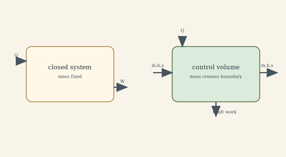
1. State, Equilibrium, and Microscopic Meaning
A macrostate is described by measurable variables such as (T,p,V,U,H,S). A microstate is the detailed particle arrangement and motion compatible with that macrostate.
For a simple compressible single-component equilibrium system,
\[U=U(S,V,N),\]and
\[T=\left(\frac{\partial U}{\partial S}\right)_{V,N}, \qquad p=-\left(\frac{\partial U}{\partial V}\right)_{S,N}, \qquad \mu=\left(\frac{\partial U}{\partial N}\right)_{S,V}.\]Temperature, pressure, and chemical potential are therefore slopes of the energy surface. They are not arbitrary labels.
Entropy has a statistical interpretation:
\[S=k_B\ln\Omega,\]where (\Omega) is the number of accessible microstates. Entropy increase is not a moral preference for disorder; it is the overwhelming statistical tendency of macroscopic systems to move toward macrostates with many compatible microstates.
Engineering thermodynamics often assumes local equilibrium: each small material element is close enough to equilibrium that (T,p,s) are meaningful even while the whole field evolves.
2. First Law: Energy Accounting
Heat and work are not stored. They are boundary transfers. A system stores internal energy, kinetic energy, potential energy, chemical energy, and other state-dependent forms.
For a closed system,
\[\Delta U+\Delta KE+\Delta PE=Q-W.\]For quasi-equilibrium boundary work,
\[W_b=\int_{V_1}^{V_2}p\,dV.\]For a steady one-inlet, one-outlet control volume,
\[\dot Q-\dot W_s = \dot m\left[(h_2-h_1)+\frac{V_2^2-V_1^2}{2}+g(z_2-z_1)\right].\]Enthalpy,
\[h=u+pv,\]packages internal energy and flow work. That is why turbines, compressors, nozzles, pumps, and heat exchangers are naturally written using (h).
At continuum scale, a representative internal-energy equation is
\[\rho\frac{De}{Dt} =-\nabla\cdot\mathbf{q} -p\nabla\cdot\mathbf{u} +\boldsymbol{\tau}:\nabla\mathbf{u} +\dot q_v.\]The terms are conduction, compressive work, viscous dissipation, and volumetric heating. This is where thermodynamics becomes field physics.
3. Second Law, Entropy, and Exergy
The first law says energy is conserved. The second law says energy quality degrades.
For any cycle,
\[\oint \frac{\delta Q}{T}\le 0.\]For a control volume,
\[\frac{dS_{cv}}{dt} = \sum \dot m_{in}s_{in} -\sum \dot m_{out}s_{out} +\sum\frac{\dot Q_k}{T_k} +\dot S_{gen}, \qquad \dot S_{gen}\ge 0.\]Entropy generation comes from finite-temperature heat transfer, friction, mixing, electrical resistance, chemical reaction away from equilibrium, shocks, and unrestrained expansion.
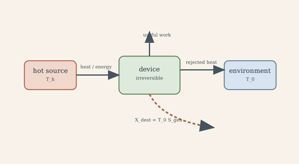
Exergy measures maximum useful work relative to an environment. A common specific flow exergy is
\[b=(h-h_0)-T_0(s-s_0)+\frac{V^2}{2}+gz.\]The exergy destruction relation is
\[\dot X_{dest}=T_0\dot S_{gen}.\]This equation is a design compass: it tells us where useful work potential is being destroyed.
4. Thermodynamic Potentials and Material Response
For a simple compressible system,
\[dU=T\,dS-p\,dV+\mu\,dN.\]Legendre transforms choose the natural potential for the constraints:
\[H=U+pV,\qquad A=U-TS,\qquad G=U+pV-TS.\]Their differentials are
\[dH=T\,dS+V\,dp+\mu\,dN,\] \[dA=-S\,dT-p\,dV+\mu\,dN,\] \[dG=-S\,dT+V\,dp+\mu\,dN.\]At fixed (T,p), spontaneous evolution tends to reduce Gibbs free energy (G). This is why (G) controls phase equilibrium and many chemical/material processes.
Response functions include
\[c_v=\left(\frac{\partial u}{\partial T}\right)_v,\qquad c_p=\left(\frac{\partial h}{\partial T}\right)_p,\] \[\alpha=\frac{1}{V}\left(\frac{\partial V}{\partial T}\right)_p,\qquad \kappa_T=-\frac{1}{V}\left(\frac{\partial V}{\partial p}\right)_T.\]One useful identity is
\[c_p-c_v=\frac{TV\alpha^2}{\kappa_T}.\]It links heat capacity difference to thermal expansion and compressibility. The table value (c_p) is therefore not isolated data; it reflects microscopic degrees of freedom and macroscopic response.
5. Real Substances and Phase Change
The ideal gas law
\[pv=RT\]works when density is low and interactions are weak. Real fluids use a compressibility factor:
\[pv=ZRT.\]Two phases coexist when temperature, pressure, and chemical potential are compatible across the interface. Along a saturation curve,
\[\frac{dp_{sat}}{dT}=\frac{h_{fg}}{T(v_g-v_f)}.\]For vaporization with (v_g\gg v_f) and near-ideal vapor,
\[\frac{d\ln p_{sat}}{dT}\approx\frac{h_{fg}}{RT^2}.\]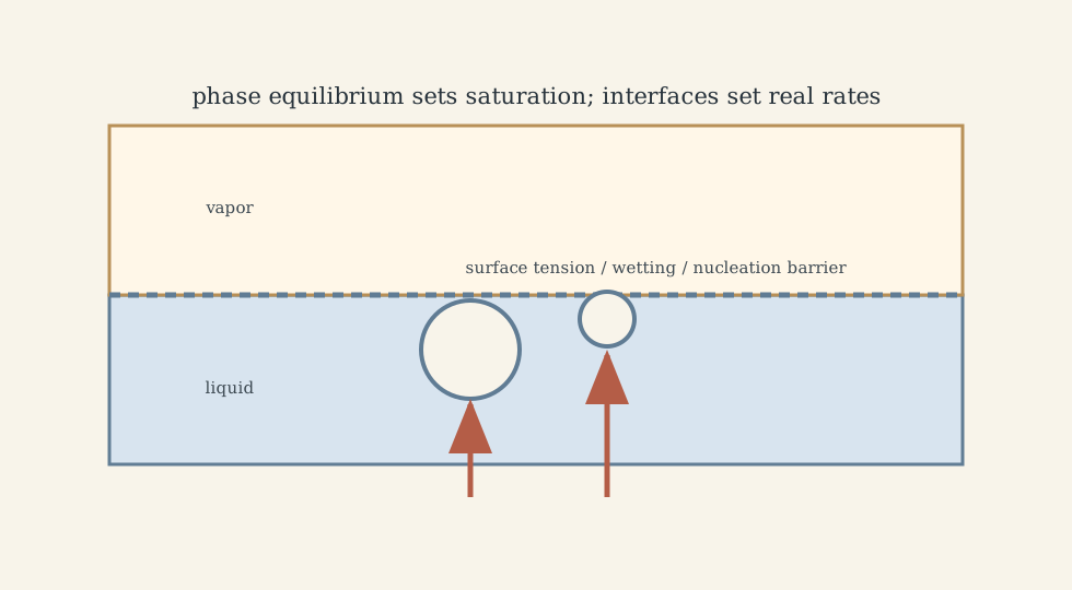
Phase change is powerful because latent heat is large. It is dangerous because regimes can change abruptly: nucleate boiling can transfer heat efficiently, while film boiling can insulate the surface and trigger overheating after critical heat flux.
6. Heat Transfer as Transport Physics
Thermodynamics says what states are possible. Heat transfer says how fast temperature fields evolve.
Fourier conduction is
\[\mathbf{q}=-k\nabla T.\]Thermal diffusivity is
\[\alpha_{th}=\frac{k}{\rho c}.\]For a stationary medium with constant properties,
\[\rho c\frac{\partial T}{\partial t} =k\nabla^2T+\dot q_v,\]or
\[\frac{\partial T}{\partial t} =\alpha_{th}\nabla^2T+\frac{\dot q_v}{\rho c}.\]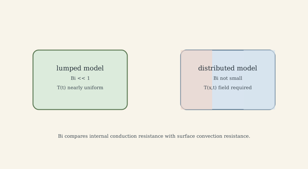
The Biot number
\[Bi=\frac{hL_c}{k}\]compares internal conduction resistance to surface convection resistance. If (Bi\ll1), a lumped-capacitance ODE may be valid. The Fourier number
\[Fo=\frac{\alpha_{th}t}{L_c^2}\]measures transient diffusion progress.
7. Convection, Radiation, and Dimensionless Groups
Convection couples flow and heat transfer. Core dimensionless groups are
\[Re=\frac{\rho UL}{\mu},\qquad Pr=\frac{\nu}{\alpha_{th}},\qquad Pe=Re\,Pr,\] \[Nu=\frac{hL}{k},\qquad Gr=\frac{g\beta\Delta T L^3}{\nu^2},\qquad Ra=Gr\,Pr.\]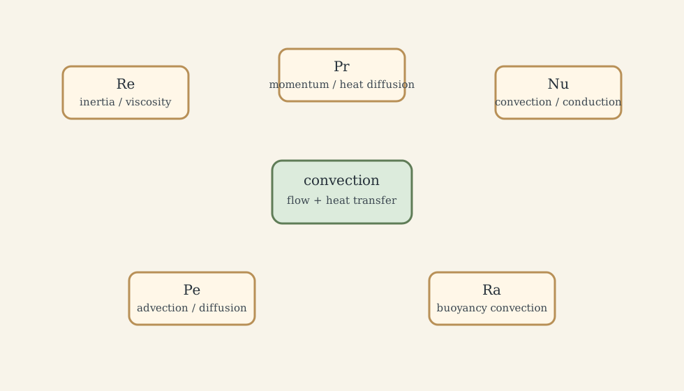
These numbers are regime tests:
- (Re): inertia versus viscosity;
- (Pr): momentum diffusion versus thermal diffusion;
- (Pe): advection versus thermal diffusion;
- (Nu): convection enhancement over pure conduction;
- (Ra): buoyancy-driven convection tendency.
Thermal radiation obeys the blackbody relation
\[E_b=\sigma T^4,\]and, in a simple gray-surface exchange approximation,
\[q=\epsilon\sigma A(T_s^4-T_{sur}^4).\]Radiation is nonlinear, spectral, and geometry-dependent. At high temperature it can dominate conduction and convection.
8. Cycles, Devices, and Limits
Ideal cycles are skeletons, not real machines. Carnot, Otto, Diesel, Brayton, and Rankine cycles reveal how heat addition, compression, expansion, and rejection are organized. Real devices add friction, pressure loss, finite-rate heat transfer, leakage, material temperature limits, and off-design control.
For a heat engine between reservoirs,
\[\eta \le 1-\frac{T_c}{T_h}.\]For refrigerators and heat pumps,
\[COP_R=\frac{Q_L}{W_{in}}, \qquad COP_{HP}=\frac{Q_H}{W_{in}}.\]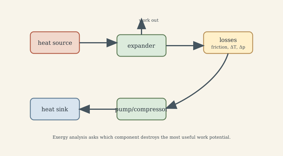
The master-level question is not only “what is efficiency?” It is:
- where is entropy generated?
- which component destroys the most exergy?
- what active constraint dominates: material temperature, pressure drop, combustion chemistry, heat-transfer area, control stability, or cost?
9. Coupled and Nonequilibrium Thermal Physics
Real systems operate with gradients and coupled fluxes. A local entropy balance can be written as
\[\rho\frac{Ds}{Dt}+\nabla\cdot\mathbf{J}_s=\sigma_s, \qquad \sigma_s\ge0.\]Near equilibrium, linear irreversible thermodynamics writes
\[J_i=\sum_j L_{ij}X_j,\]where (J_i) are fluxes and (X_j) are thermodynamic forces. Under suitable symmetry assumptions,
\[L_{ij}=L_{ji}.\]This language explains thermoelectricity, coupled heat/mass diffusion, porous-media transport, electrochemical heating, and reacting-flow coupling.
Thermal physics also couples directly to:
- fluids: buoyancy, compressibility, turbulence, combustion, boiling;
- solids: thermal stress, shock, residual stress, packaging failure;
- materials: phonon/electron transport, phase transformations, porosity;
- chemistry: reaction enthalpy, kinetics, species diffusion.
Constrained thermal strain is
\[\epsilon_{th}=\alpha_T\Delta T,\]and if that strain cannot relax, thermal stress follows. This is why thermal analysis is inseparable from mechanics in welding, brakes, turbine blades, electronics, and additive manufacturing.
10. Modeling Hierarchy
Choose the simplest model that captures the dominant mechanism:
- Equilibrium thermodynamics for state changes, ideal limits, and property bookkeeping.
- Lumped dynamic models when spatial gradients are weak and (Bi\ll1).
- Distributed transport models when temperature, velocity, or concentration vary in space.
- Multiphysics models when phase change, radiation, reaction, deformation, or microstructure dominate.
The mature question is not “what is the most advanced model?” It is:
- which term dominates?
- which constitutive relation is uncertain?
- which approximation sets the error floor?
- which measurement would falsify the model fastest?
What This Framework Lets Us Do
This framework lets us connect thermodynamics, heat transfer, fluids, materials, and energy systems:
- energy balances say what is conserved;
- entropy balances say what direction is possible and what work potential is lost;
- potentials say which state changes are spontaneous under constraints;
- transport equations say how fast fields evolve;
- dimensionless groups say which regime we are in;
- exergy says where redesign effort matters.
Where the Framework Stops Being Reliable
It fails when assumptions are violated: non-equilibrium too strong for local (T,p,s), correlations used outside range, ideal gas models used in dense or two-phase regions, constant properties used across large temperature spans, radiation geometry ignored, or thermal coupling to stress/chemistry/flow neglected.
Where the Subject Leads Next
Thermal dynamics leads to fluid dynamics, combustion, electronics cooling, building physics, heat exchangers, turbomachinery, phase-change systems, batteries, materials processing, and climate/energy systems.
Compact Recall Map
- Define the system boundary before writing balances.
- Heat and work are transfers; internal energy is stored.
- Entropy generation marks irreversibility.
- Exergy identifies destroyed useful work potential.
- Phase equilibrium is thermodynamic; boiling and condensation are interfacial transport.
- Heat conduction is diffusion of thermal energy.
- Convection is heat transfer coupled to flow.
- Radiation is nonlinear and geometry-dependent.
- Dimensionless groups determine regime and model validity.
- Real thermal systems are usually multiphysics.
Technical and Editorial Audit
| Area | Correction or decision |
|---|---|
| Central question | Reframed thermal dynamics around state, energy, entropy, transport, exergy, and model hierarchy. |
| Preserved equations | Kept state derivatives, first-law balances, entropy balance, potentials, response functions, phase relations, heat equation, dimensionless groups, radiation, cycle limits, exergy, entropy production, and thermal strain. |
| Units and assumptions | Clarified boundary types, local equilibrium, lumped validity, ideal-gas limits, and regime dependence of correlations. |
| Figures | Added six original SVG diagrams for boundaries, entropy/exergy, phase change, lumped/distributed models, convection groups, and cycle exergy losses. |
| Editorial correction | Reduced dense theorem-like sequencing and reorganized around engineering questions and model validity. |
Main Sources Used in This Note
- CityU MNE2112 and MNE3121 course material.
- Standard references such as Cengel and Boles, Thermodynamics, and Incropera et al., Fundamentals of Heat and Mass Transfer.