Biology Modelling Notes
This note is adapted from course materials for 1BG383 Modelling in Biology at Uppsala University. Instructor: course teaching staff.
Central Question
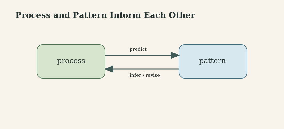
Biological modelling asks: which mechanisms could have produced the pattern we observe, and what patterns should follow if our mechanism is right?
The core loop is
\[\text{process}\Longleftrightarrow\text{pattern}.\]Models can run forward from assumptions to predictions, or backward from observations to plausible mechanisms. Their value is not that they make biology simple. Their value is that they make assumptions explicit.
1. Building a Dynamic Model
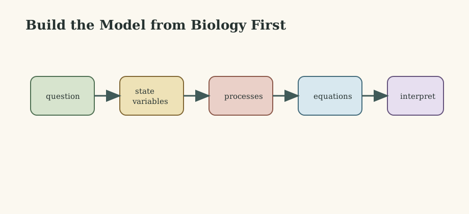
A dynamic model needs state variables, processes, parameters, and time representation. A state vector is
\[x(t)=(x_1(t),x_2(t),\ldots,x_n(t)).\]Discrete-time models use recursions:
\[x(t+1)=F(x(t)).\]Continuous-time models use differential equations:
\[\frac{dx}{dt}=f(x).\]The choice should follow biology. Seasonal reproduction, annual census data, and pulsed life cycles often fit discrete time. Continuous growth, infection, movement, and physiological rates often fit continuous time.
2. Population Growth and Regulation
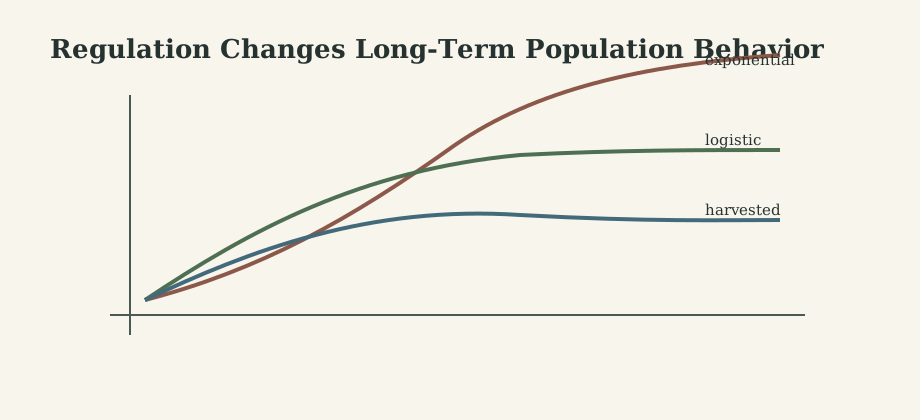
Exponential growth assumes per-capita change is constant:
\[\frac{dN}{dt}=rN.\]It is useful locally but unrealistic as a long-run model. Logistic growth adds density regulation:
\[\frac{dN}{dt}=rN\left(1-\frac{N}{K}\right).\]Here $r$ is intrinsic growth rate and $K$ is carrying capacity. The equilibria are $N=0$ and $N=K$, and growth is maximal at $N=K/2$.
Harvesting changes the qualitative dynamics:
\[\frac{dN}{dt}=N(r-\alpha N)-EN.\]The management question is not only the final population size. It is whether exploitation changes stability, creates collapse thresholds, or removes biologically meaningful equilibria.
3. Epidemic Compartment Models
The baseline SIR model is
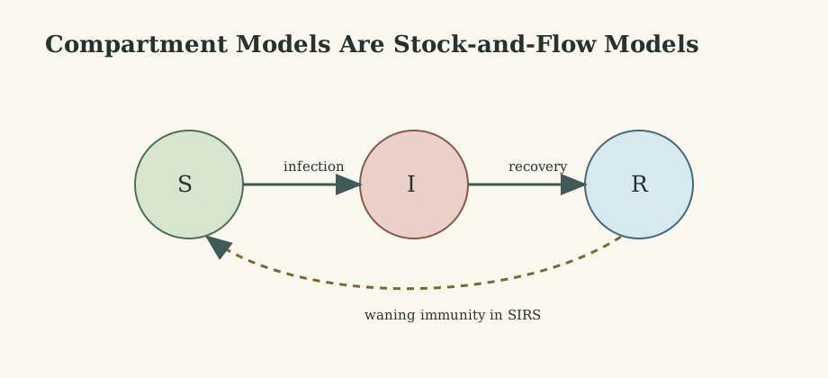
\[\frac{dS}{dt}=-\frac{b}{N}SI,\] \[\frac{dI}{dt}=\frac{b}{N}SI-\frac{I}{T_r},\] \[\frac{dR}{dt}=\frac{I}{T_r}.\]Susceptibles are lost through infection, infected individuals recover, and recovered individuals accumulate. Early in an outbreak, with $S\approx N$, infection grows when
\[b-\frac{1}{T_r}>0 \quad\Longleftrightarrow\quad bT_r>1.\]SIRS adds waning immunity:
\[\frac{dS}{dt}=-\frac{b}{N}SI+\frac{R}{T_i},\] \[\frac{dI}{dt}=\frac{b}{N}SI-\frac{I}{T_r},\] \[\frac{dR}{dt}=\frac{I}{T_r}-\frac{R}{T_i}.\]Vital dynamics add births and deaths. Each extension changes the biological story: outbreak fade-out, recurrent waves, or endemic persistence.
4. Stability, Phase Planes, and Bifurcation
An equilibrium satisfies
\[\frac{dx}{dt}=0 \quad\text{or}\quad x(t+1)=x(t).\]For a one-dimensional continuous model $\dot x=f(x)$, local stability near $\hat x$ depends on $f’(\hat x)$. Negative slope gives local stability; positive slope gives instability.
In multiple dimensions, the Jacobian controls local behavior:
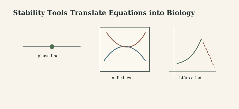
\[J(\hat x)= \left[\frac{\partial f_i}{\partial x_j}\right]_{x=\hat x}.\]Eigenvalues with negative real parts imply local stability in continuous time. In two-dimensional ecological systems, nullclines and phase planes reveal coexistence, exclusion, cycles, and basins of attraction.
Bifurcation analysis tracks how equilibria or attractors change as a parameter varies. This is essential in harvesting, epidemic thresholds, predator-prey systems, and discrete-time density dependence. Simple deterministic maps can pass from stable equilibrium to period-doubling and chaos.
5. Interactions and Functional Responses
Interaction terms encode biological assumptions. A Holling type II functional response is
\[F(R)=\frac{aR}{1+aRh},\]where $a$ is search efficiency, $h$ is handling time, and $R$ is resource density. This saturating shape says consumption is limited not only by finding prey but also by processing them.
Different functional responses can change stability and coexistence. This is why interaction terms should not be chosen only for algebraic convenience.
6. Stochasticity and Computation
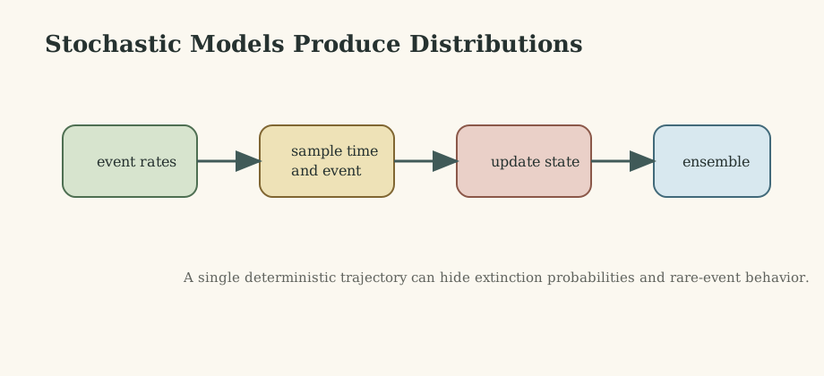
Deterministic models describe average tendencies, but biological systems include random births, deaths, environmental fluctuations, rare events, and sampling noise. In small populations, stochastic extinction can occur even when deterministic growth predicts persistence.
The Gillespie algorithm simulates stochastic event processes by sampling both the time to the next event and which event occurs. This matters for invasion biology, conservation, epidemiology, and cellular systems.
Computation in R usually follows:
- define the right-hand side,
- set parameters and initial conditions,
- solve numerically,
- sweep parameters,
- compare transients and long-run behavior,
- revise the model.
Euler’s idea is
\[x_{n+1}=x_n+\Delta t\,f(x_n),\]but production analysis should use appropriate solvers and sensitivity checks.
What This Framework Lets Us Do
Biological modelling connects verbal hypotheses, mathematical structure, simulation, and data. It helps explain population regulation, epidemic thresholds, harvesting risk, predator-prey dynamics, stochastic extinction, and theory-guided empirical work.
Where the Framework Stops Being Reliable
A model can fit data while explaining little. Parameters may be unmeasurable, mechanisms may be missing, and extrapolation can fail outside the observed regime. Deterministic stability does not remove stochastic risk.
Where the Subject Leads Next
The next steps are statistical inference for dynamic models, stochastic differential equations, agent-based models, spatial ecology, evolutionary game dynamics, Bayesian calibration, and theory-experiment integration.
Technical and Editorial Audit
- Reorganized the long course note into a process-pattern learning path.
- Preserved the 1BG383 Uppsala University course attribution in the main text.
- Added original figures for modelling loop, model construction, population regulation, epidemic compartments, stability/bifurcation, and stochastic simulation.
- Kept the central equations for discrete and continuous dynamics, logistic growth, harvesting, SIR/SIRS, stability, functional responses, and Euler integration.
- Biological claims should be checked against the empirical system before using any model for management decisions.
Main Sources Used in This Note
- S. P. Otto and T. Day, A Biologist’s Guide to Mathematical Modeling in Ecology and Evolution.
- J. D. Murray, Mathematical Biology.
- M. J. Keeling and P. Rohani, Modeling Infectious Diseases in Humans and Animals.
- N. G. van Kampen, Stochastic Processes in Physics and Chemistry.