Lie group and lie algebra for robotics
This note is adapted from local robotics materials in /mnt/d/UU/robotics/, especially the 2018 PDFs on transformations, rotations, angular velocity, twists, Kalman filtering, visual-inertial fusion, camera models, and PnP. The course-code attribution is kept in the main text rather than the front matter because the source folder contains lecture-style files but not a single unambiguous university course record for this note.
Central Question
Lie groups in robotics ask: how can we compute with rigid-body poses without pretending that rotations are ordinary Euclidean vectors?
That question shows up everywhere:
- A mobile robot composes odometry increments.
- A manipulator chains joint transforms.
- A camera estimates its pose from image features.
- An IMU integrates angular velocity and acceleration.
- A Kalman filter stores uncertainty around an orientation.
- A trajectory optimizer updates poses using local residuals.
The common mistake is to treat a pose as just another vector. Translation is vector-like, but orientation is not. A 3D rotation matrix has nine numbers and only three degrees of freedom; a quaternion has four numbers and one unit-norm constraint; Euler angles have singularities and convention traps. Lie theory is the bridge:
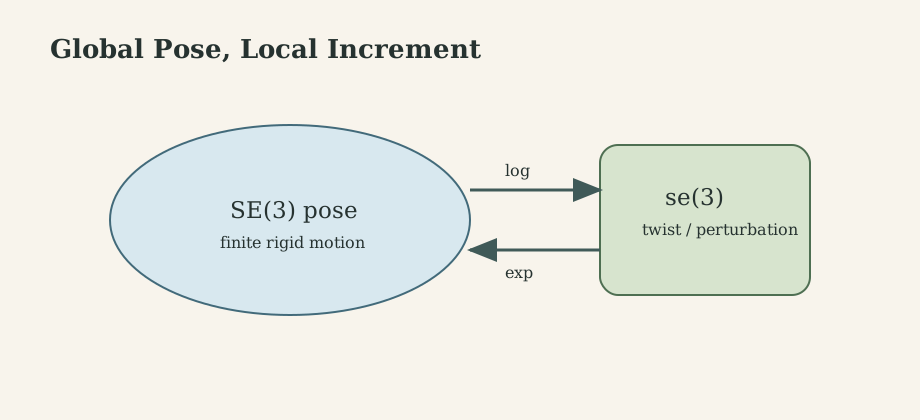
- the group describes finite motions,
- the algebra describes local perturbations and velocities,
- the exponential integrates local motion into finite motion,
- the logarithm turns finite disagreement into a local residual.
1. Frames First: Coordinates Are Not the Object
A physical vector is independent of coordinates. Its coordinate column changes when the reference frame changes. If a frame has basis vectors ${\mathbf e_1,\mathbf e_2,\mathbf e_3}$, then
\[\mathbf a = [\mathbf e_1,\mathbf e_2,\mathbf e_3] \begin{bmatrix}a_1\\a_2\\a_3\end{bmatrix}.\]For two frames $A$ and $B$, let $R_{AB}$ be the rotation whose columns are the axes of frame $B$ expressed in frame $A$. If $p_B$ is the coordinate column of a point in frame $B$, then the same point expressed in frame $A$ is
\[p_A = R_{AB}p_B + t_{AB},\]where $t_{AB}$ is the origin of frame $B$ expressed in frame $A$.
Homogeneous coordinates package rotation and translation as
\[T_{AB} = \begin{bmatrix} R_{AB} & t_{AB}\\ 0^\top & 1 \end{bmatrix}, \qquad \bar p_A = T_{AB}\bar p_B.\]The inverse is not the transpose of the whole homogeneous matrix:
\[T_{AB}^{-1} = \begin{bmatrix} R_{AB}^\top & -R_{AB}^\top t_{AB}\\ 0^\top & 1 \end{bmatrix}.\]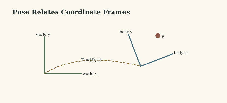
The notation $T_{AB}$ is already a convention. In this note it means “transform coordinates from frame $B$ into frame $A$.” Some libraries instead store the pose of $A$ in $B$, some write active transforms that move physical vectors, and some use row vectors. The mathematics can support all of these; the software cannot survive mixing them casually.
2. Composition: Current Frame or Fixed Frame?
Rigid-body transformations compose by matrix multiplication:
\[T_{AC}=T_{AB}T_{BC}.\]The right-hand transform acts first on coordinates. If a motion is specified relative to the current/body frame, it is typically post-multiplied. If it is specified relative to the fixed/world frame, it is typically pre-multiplied. For example, starting from $T$,
\[\text{body update:}\qquad T^+ = T\Delta T,\] \[\text{world update:}\qquad T^+ = \Delta T T.\]These two updates are not interchangeable because rotations and rigid transforms do not commute. A “move forward, then turn” command is generally different from “turn, then move forward.”
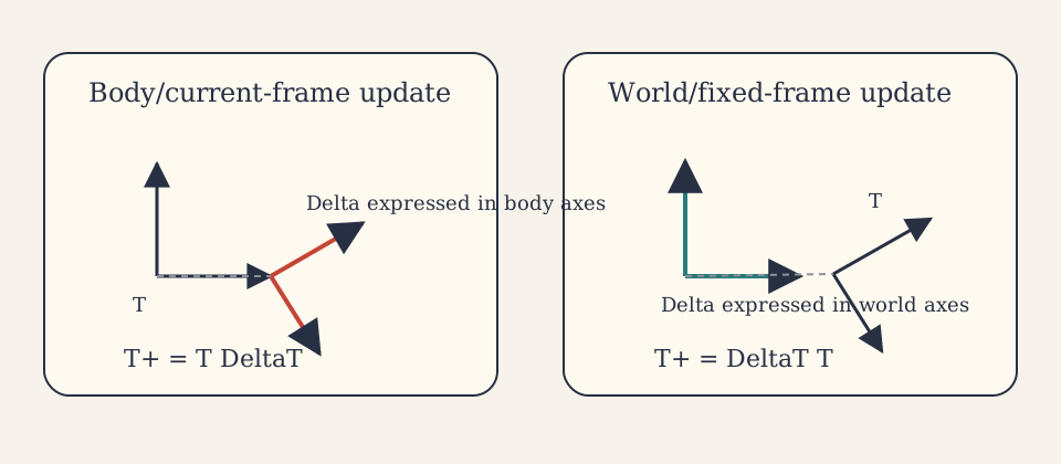
A useful debugging habit is to annotate every transform with its source and target frame. If the middle indices do not cancel in a product such as $T_{AB}T_{BC}$, the multiplication is probably wrong.
3. The Rotation Group SO(3)
Valid 3D rotation matrices form the special orthogonal group
\[SO(3) = \{R\in\mathbb R^{3\times3}\mid R^\top R=I,\ \det R=1\}.\]This set is a group:
- closure: $R_1R_2\in SO(3)$,
- identity: $I\in SO(3)$,
- inverse: $R^{-1}=R^\top$,
- associativity: inherited from matrix multiplication.
It is also a smooth manifold. This matters because $SO(3)$ is curved inside $\mathbb R^9$. Its valid elements satisfy six independent orthogonality constraints and one orientation constraint, leaving three degrees of freedom. You can use three local coordinates, but no single global three-parameter chart is perfect.
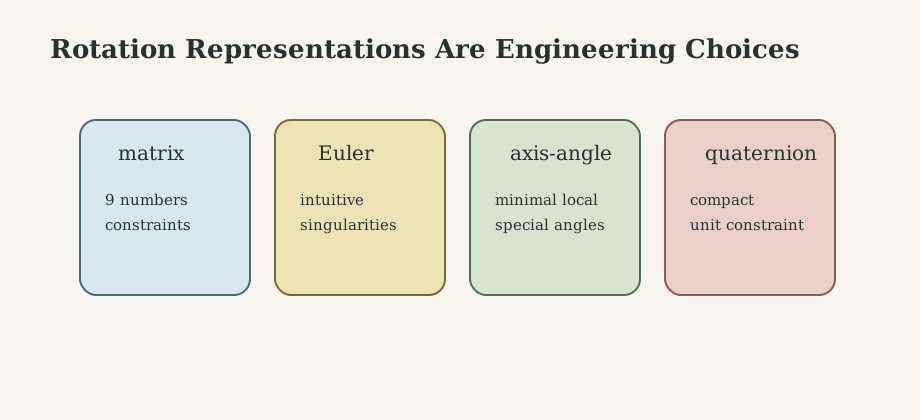
Common rotation representations are all compromises:
- Rotation matrices are globally nonsingular but redundant and constrained.
- Euler angles are compact and human-readable but convention-heavy and singular.
- Axis-angle is geometrically clear but has ambiguity at $\theta=\pi$ and undefined axis at $\theta=0$.
- Unit quaternions avoid gimbal lock and integrate well, but $q$ and $-q$ represent the same rotation.
- Exponential coordinates are ideal for local increments, but the logarithm needs care near $\pi$.
Euler-angle warnings are not just mathematical trivia. A controller that maps Euler-angle rates to angular velocity can become singular when axes align. The angular velocity of the rigid body is not generally the time derivative of a chosen Euler-angle vector.
4. The Algebra so(3): Cross Products as Matrices
The tangent space of $SO(3)$ at the identity is the Lie algebra $\mathfrak{so}(3)$, the set of skew-symmetric matrices:
\[\mathfrak{so}(3) = \{\phi^\wedge\mid \phi\in\mathbb R^3\},\]with the wedge operator
\[\phi^\wedge = \begin{bmatrix} 0 & -\phi_3 & \phi_2\\ \phi_3 & 0 & -\phi_1\\ -\phi_2 & \phi_1 & 0 \end{bmatrix}.\]It satisfies
\[\phi^\wedge x = \phi\times x.\]For a unit axis $u$ and angle $\theta$, Rodrigues’ formula gives
\[\exp(u^\wedge\theta) = I +u^\wedge\sin\theta +(u^\wedge)^2(1-\cos\theta).\]This is the 3D version of the familiar 2D idea $e^{i\theta}=\cos\theta+i\sin\theta$: a tangent-space quantity exponentiates to a rotation. The logarithm reverses this locally by extracting an axis and an angle from a rotation matrix.
The Lie bracket is the matrix commutator:
\[[A,B]=AB-BA.\]For $\mathfrak{so}(3)$ this corresponds to the vector cross product:
\[[\phi^\wedge,\psi^\wedge] = (\phi\times\psi)^\wedge.\]5. Angular Velocity: Spatial Versus Body
Differentiating $R^\top R=I$ shows that $R^\top \dot R$ and $\dot R R^\top$ are skew-symmetric. Therefore they correspond to angular-velocity vectors:
\[\omega_b^\wedge = R^\top\dot R, \qquad \omega_s^\wedge = \dot R R^\top.\]The subscripts are important:
- $\omega_b$ is angular velocity expressed in the body frame.
- $\omega_s$ is angular velocity expressed in the spatial/world frame.
They are related by
\[\omega_s = R\omega_b.\]The rotation kinematics can be written in either convention:
\[\dot R = R\omega_b^\wedge \qquad\text{or}\qquad \dot R = \omega_s^\wedge R.\]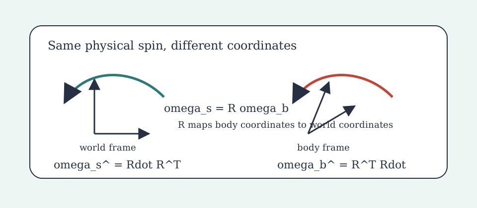
This is one of the places where robotics notation earns its keep. If an IMU reports angular velocity in the sensor/body frame, integrating it as if it were world-frame angular velocity creates a slowly poisonous estimator.
6. SE(3): Rigid Poses as a Lie Group
Rigid-body poses in 3D form
\[SE(3) = \left\{ \begin{bmatrix} R&t\\ 0^\top&1 \end{bmatrix} \middle| R\in SO(3),\ t\in\mathbb R^3 \right\}.\]The group operation is homogeneous-matrix multiplication:
\[\begin{bmatrix} R_1&t_1\\ 0^\top&1 \end{bmatrix} \begin{bmatrix} R_2&t_2\\ 0^\top&1 \end{bmatrix} = \begin{bmatrix} R_1R_2 & R_1t_2+t_1\\ 0^\top&1 \end{bmatrix}.\]This noncommutative product is the reason rigid-body pose is not just “three for rotation plus three for translation.” Translation is rotated during composition. That coupling is exactly what makes the group structure useful for odometry chains, camera extrinsics, manipulator kinematics, and pose graphs.
7. Twists and se(3)
The Lie algebra $\mathfrak{se}(3)$ contains twists. With the linear-then-angular convention
\[\xi = \begin{bmatrix} \rho\\ \phi \end{bmatrix} \in\mathbb R^6,\]the wedge operator is
\[\xi^\wedge = \begin{bmatrix} \phi^\wedge & \rho\\ 0^\top & 0 \end{bmatrix}.\]The exponential map turns a twist increment into a finite rigid-body transform:
\[\operatorname{Exp}(\xi)=\exp(\xi^\wedge)\in SE(3).\]The logarithm turns a relative transform into a six-dimensional local displacement:
\[\operatorname{Log}(T)=\xi\in\mathbb R^6.\]For a time-varying pose $T(t)$, the spatial twist matrix is
\[\xi_s^\wedge = \dot T T^{-1},\]so that
\[\dot T = \xi_s^\wedge T.\]The body twist matrix is
\[\xi_b^\wedge = T^{-1}\dot T,\]so that
\[\dot T = T\xi_b^\wedge.\]The two are the same physical rigid-body velocity expressed in different frames.
8. The Adjoint: Moving Velocities and Perturbations Between Frames
The adjoint representation maps twists between frames. For
\[T= \begin{bmatrix} R&t\\ 0^\top&1 \end{bmatrix},\]and twist order $\xi=[\rho^\top,\phi^\top]^\top$, one common convention is
\[\operatorname{Ad}_T = \begin{bmatrix} R&t^\wedge R\\ 0&R \end{bmatrix}.\]Then
\[\xi_s = \operatorname{Ad}_T\xi_b.\]The algebra adjoint is
\[\operatorname{ad}_{\xi} = \begin{bmatrix} \phi^\wedge & \rho^\wedge\\ 0&\phi^\wedge \end{bmatrix},\]and it satisfies
\[\operatorname{Ad}_{\operatorname{Exp}(\xi)} = \exp(\operatorname{ad}_{\xi}).\]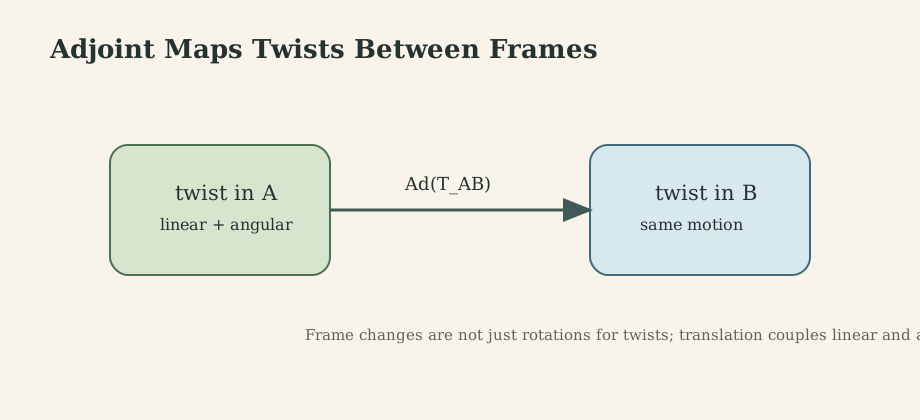
The adjoint also tells you how uncertainty changes frames. If a covariance $P_b$ is expressed in body-frame tangent coordinates, the corresponding spatial-frame covariance is approximately
\[P_s = \operatorname{Ad}_T P_b \operatorname{Ad}_T^\top.\]9. Box-Plus, Box-Minus, and Jacobians on Manifolds
Most optimization and filtering code wants vector increments. Lie groups provide vector increments without leaving the pose manifold.
With a right perturbation convention,
\[T\oplus\delta := T\operatorname{Exp}(\delta),\]and a right-invariant residual can be written
\[T_2\ominus T_1 := \operatorname{Log}(T_1^{-1}T_2).\]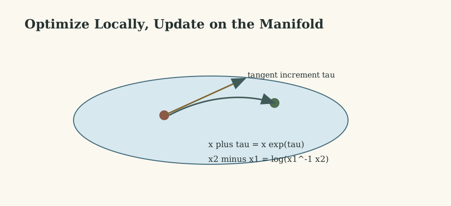
The manifold derivative of a function $f$ is not the plain derivative of matrix entries. It is a derivative through the chosen plus and minus operations:
\[J = \frac{Df(x)}{Dx} = \lim_{\delta\to0} \frac{f(x\oplus\delta)\ominus f(x)}{\delta}.\]Covariance propagation is then performed in tangent coordinates:
\[P_y \approx J P_x J^\top.\]This is why left/right perturbation choices matter. A Jacobian derived for $T^+=T\operatorname{Exp}(\delta)$ is not automatically correct for $T^+=\operatorname{Exp}(\delta)T$.
10. Estimation: From Bayes Filters to Error-State EKF
The filtering materials in the robotics folder make the same geometric point from a probabilistic direction. A Bayes or Kalman filter needs a complete state so that the future is conditionally independent of the deeper past once the current state and input are known. For a moving robot, position alone is often not complete; velocity, orientation, and sensor biases may be part of the state.
A typical visual-inertial state is
\[x = \{p,\ v,\ q,\ b_g,\ b_a,\ g\},\]where $p$ is position, $v$ is velocity, $q$ is orientation, $b_g$ and $b_a$ are gyroscope and accelerometer biases, and $g$ is gravity. Most components can be perturbed by addition, but orientation is perturbed by composition:
\[q^+ = q\otimes\delta q.\]For a small rotation error $\delta\theta$,
\[\delta q \approx \begin{bmatrix} 1\\ \frac{1}{2}\delta\theta \end{bmatrix}.\]This is the heart of an error-state EKF: the nominal state carries the actual pose-like quantities, while the filter covariance lives in a local error vector. Prediction integrates IMU measurements; update compares predicted measurements with camera observations; correction injects a small tangent-space error back into the nominal state.
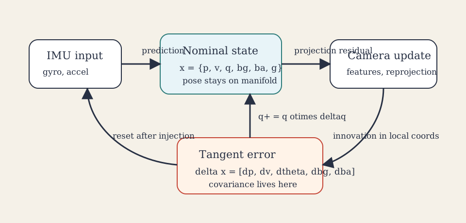
The innovation must also respect geometry. For Euclidean position, an innovation can be a subtraction. For orientation, the innovation should be a logarithm of a relative rotation, not a naive component-wise quaternion difference.
11. Camera Geometry and Pose Estimation
Computer vision adds another layer of coordinate discipline. A calibrated pinhole camera maps a 3D point in camera coordinates to an image ray. With camera intrinsics $K$ and a camera pose $T_{CW}$ that maps world coordinates into camera coordinates,
\[\lambda \begin{bmatrix} u\\v\\1 \end{bmatrix} = K \begin{bmatrix} I&0 \end{bmatrix} T_{CW} \begin{bmatrix} X_W\\1 \end{bmatrix}.\]The scalar $\lambda$ is depth. The image measurement gives a ray, not a full 3D point, unless depth or multiple-view constraints are available.
Pose-from-points problems such as PnP estimate camera pose from 2D-3D correspondences. Fiducials such as AprilTags make the geometry concrete: known points in a tag frame are observed in the image, and the camera pose is estimated by minimizing reprojection error. In a filter, the residual belongs in the measurement space, while the pose correction belongs in the tangent space of $SE(3)$ or $SO(3)$.
This is where Lie groups connect camera models, IMU integration, and filtering:
- IMU prediction integrates body-frame angular velocity and acceleration.
- Camera update constrains pose through projection geometry.
- The estimator stores orientation uncertainty as a local three-vector.
- The pose update uses group composition instead of raw vector addition.
12. Practical Robotics Checklist
When implementing these ideas, I want the following checklist near the code:
- Define whether $T_{AB}$ maps coordinates from $B$ to $A$ or stores the pose of $A$ in $B$.
- Define whether perturbations are left or right perturbations.
- Define whether twist vectors are ordered as linear-then-angular or angular-then-linear.
- Define whether angular velocities are spatial/world-frame or body/sensor-frame.
- Normalize quaternions after numerical integration, but do not use normalization as a substitute for correct dynamics.
- Use $\operatorname{Log}(R_1^\top R_2)$ or $\operatorname{Log}(T_1^{-1}T_2)$ for rotational or pose residuals.
- Keep covariance in tangent coordinates, not in raw matrix entries.
- For camera models, keep track of whether the pose maps world to camera or camera to world.
- Test transform code with nonzero rotation and translation; pure translations hide frame-order mistakes.
13. What This Framework Lets Us Do
Lie groups make robotics calculations compositional. They let us chain frames, integrate angular velocity, express rigid-body velocity as twists, transform velocity and uncertainty between frames, compute camera pose residuals, and optimize trajectories without violating rotation constraints.
They also explain why robotics code can look “almost right” while being badly wrong. The formulas are short, but every formula carries a convention. Most bugs come not from forgetting $SO(3)$ exists, but from mixing body and world frames, active and passive transforms, or left and right perturbations.
14. Where the Subject Leads Next
The natural next topics are:
- manipulator Jacobians and screw theory,
- pose-graph SLAM,
- invariant EKFs,
- visual-inertial odometry,
- bundle adjustment on manifolds,
- Lie-group variational integration,
- trajectory optimization on $SE(3)$.
The core pattern remains the same: compute finite poses on the group, compute small errors in the algebra, and state conventions so clearly that future-you cannot accidentally change them.
Technical and Editorial Audit
- Deepened the note from a compact Lie-theory summary into a robotics workflow: frames, transformations, rotation representations, angular velocity, twists, adjoints, manifold Jacobians, filtering, VIO, camera geometry, and implementation checks.
- Incorporated material from the local robotics PDFs on transformations, rotations, angular velocities, twists, Kalman filtering, visual-inertial fusion, camera models, and PnP.
- Preserved the existing local figure set and added original SVGs for composition conventions, body/spatial angular velocity, and error-state visual-inertial estimation.
- Kept one explicit twist convention: $\xi=[\rho^\top,\phi^\top]^\top$, meaning linear part first and angular part second.
- Flagged convention dependence as the highest practical risk: transform direction, active/passive interpretation, left/right perturbations, twist ordering, and quaternion ordering differ across libraries.
Main Sources Used in This Note
- Local robotics materials in
/mnt/d/UU/robotics/:01_2018_transformations.pdf,02_2018_rotations.pdf,03_2018_rotations_velocities.pdf,04_2018_travelocities.pdf,11_2018_bayesianfiltering.pdf,12_2018_kalmanfilter.pdf,14_2018_visual_inertial.pdf,15_2018-extended_kalman_filter.pdf,cameramodel2018.pdf, andpnp2018.pdf. - T. D. Barfoot, State Estimation for Robotics.
- J. Sola, J. Deray, and D. Atchuthan, “A micro Lie theory for state estimation in robotics.”
- R. M. Murray, Z. Li, and S. S. Sastry, A Mathematical Introduction to Robotic Manipulation.
- E. Eade, Lie Groups for 2D and 3D Transformations.