Adaptive, Optimal, Robust, and Learning Control
This note is a Uppsala University advanced course for PhD, instructor: Dr. Christos Verginis and Dr. Aris Kanellopoulos.
Central Question
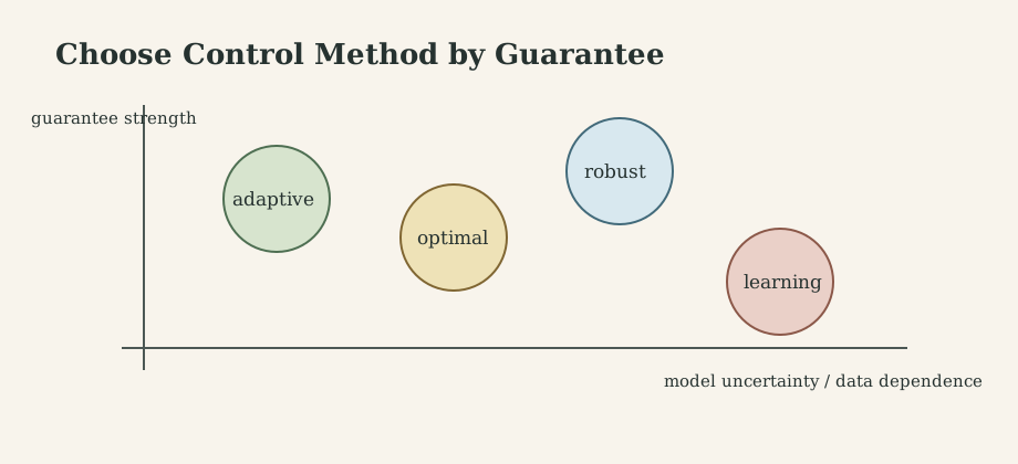
Advanced control asks: what kind of uncertainty is present, and what kind of guarantee do we need?
Adaptive, optimal, robust, and learning control are not interchangeable labels. They answer different engineering questions:
- adaptive control learns structured uncertainty online,
- optimal control optimizes a model and cost,
- robust control protects against modeled uncertainty sets,
- reinforcement learning estimates policies or values from data and interaction.
This note builds on Control Theory Basics, Modern, Multivariable, and Networked Control, and Topics in Nonlinear Systems.
1. Lyapunov Toolkit and Proof Logic
Many advanced-control proofs begin with a nonlinear system
\[\dot x=f(t,x,u), \qquad x(t_0)=x_0.\]If $f$ is locally Lipschitz in $x$ and trajectories stay bounded, continuation arguments prevent finite escape. This is why proofs often first establish boundedness and only then discuss convergence.
A Lyapunov function $V(x)$ translates dynamics into an energy-like inequality:
\[\alpha_1(\|x\|)\le V(x)\le \alpha_2(\|x\|), \qquad \dot V\le -W(x).\]This gives boundedness and convergence to the largest invariant set where $W(x)=0$. For non-autonomous adaptive systems, the usual Barbalat pattern is:
\[g\in L_2\cap L_\infty,\qquad \dot g\in L_\infty \quad \Rightarrow \quad g(t)\to0.\]The proof discipline is the same throughout the note: state assumptions, build a certificate, cancel or bound cross terms, then state exactly what is guaranteed.
2. Model Reference Adaptive Control
Model Reference Adaptive Control asks a plant to track a chosen reference model. For
\[\dot x=Ax+Bu,\qquad \dot x_m=A_mx_m+B_mr,\]with $A_m$ Hurwitz and tracking error $e=x-x_m$, a typical controller is
\[u=K_x^\top x+K_r^\top r.\]Under exact matching assumptions, a composite Lyapunov function is
\[V=e^\top Pe+ \operatorname{tr}(\tilde K_x^\top\Gamma_x^{-1}\tilde K_x)+ \operatorname{tr}(\tilde K_r^\top\Gamma_r^{-1}\tilde K_r),\]where
\[A_m^\top P+PA_m=-Q,\qquad Q>0.\]Choosing
\[\dot K_x=-\Gamma_xxe^\top PB,\qquad \dot K_r=-\Gamma_rre^\top PB\]cancels parameter-error cross terms and yields
\[\dot V=-e^\top Qe\le0.\]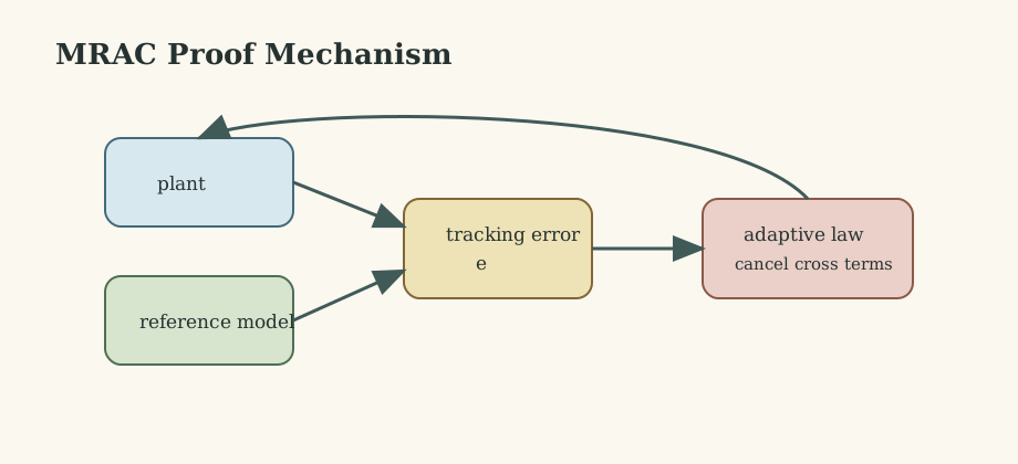
The guarantee is boundedness and tracking-error convergence under assumptions. It is not automatic parameter identification. Parameter convergence usually requires persistent excitation:
\[\int_t^{t+T}\phi(\tau)\phi(\tau)^\top d\tau\ge \alpha I.\]3. Robust Adaptive Modifications
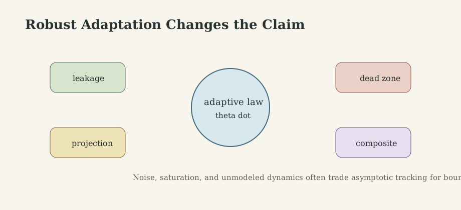
Ideal adaptation is fragile under noise, unmodeled dynamics, saturation, and weak excitation. Robust modifications adjust the theorem being proved.
Sigma modification adds leakage:
\[\dot\theta=-\Gamma\phi e-\sigma\theta,\qquad \sigma>0.\]Projection keeps estimates in a feasible set. Dead zones stop adaptation when error is dominated by noise. Normalization avoids excessively large updates when regressors become large. Composite adaptation adds prediction-error information:
\[\dot{\hat\theta}=-\Gamma(Y^\top e+W^\top\epsilon_p).\]The trade is usually better robustness for weaker asymptotic claims, often uniform ultimate boundedness rather than exact convergence.
4. Optimal Feedback: PMP, HJB, LQR, and MPC
Finite-horizon optimal control solves
\[\min_{u(\cdot)} \phi(x(t_f))+\int_{t_0}^{t_f}L(x,u,t)\,dt\]subject to
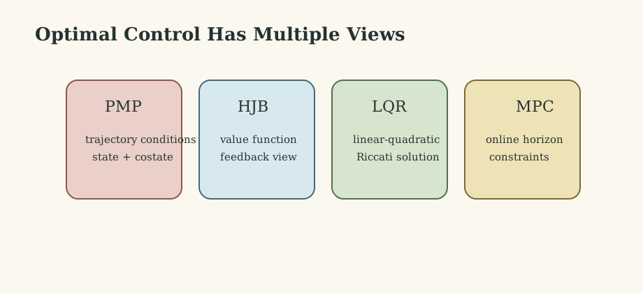
\[\dot x=f(x,u,t).\]Pontryagin’s minimum principle introduces the Hamiltonian
\[H=L+\lambda^\top f\]and necessary conditions
\[\dot x=\frac{\partial H}{\partial\lambda},\qquad \dot\lambda=-\frac{\partial H}{\partial x},\qquad u^*\in\arg\min_u H.\]The HJB equation gives a feedback view:
\[-\partial_tV=\min_u\{L+\nabla_xV^\top f\}.\]For LQR,
\[\dot x=Ax+Bu,\qquad J=\int_0^\infty(x^\top Qx+u^\top Ru)\,dt,\]the optimal law is
\[u^*=-R^{-1}B^\top Px,\]where $P$ solves the algebraic Riccati equation. MPC wraps finite-horizon optimization in feedback by repeatedly solving, applying only the first input, and shifting the horizon.
5. Robust Control and Disturbance Rejection
Robust control asks what survives worst-case uncertainty. The $H_\infty$ viewpoint minimizes the largest closed-loop amplification from disturbance to performance output. Structured uncertainty leads toward $\mu$-analysis and synthesis.
Adaptive control says “learn structured uncertainty while staying stable.” Robust control says “guarantee performance for every plant in this uncertainty set.” ADRC estimates a lumped disturbance through an extended-state observer. Each is valuable, but each encodes a different uncertainty story.
6. Reinforcement Learning in Feedback Systems
In discrete decision problems, dynamic programming uses Bellman recursion:
\[V^*(s)=\max_a\left[r(s,a)+\gamma\sum_{s'}P(s'|s,a)V^*(s')\right].\]Reinforcement learning replaces exact models with samples and approximation. In continuous control, actor-critic methods can be read as approximate HJB methods: the critic estimates value, and the actor estimates policy.
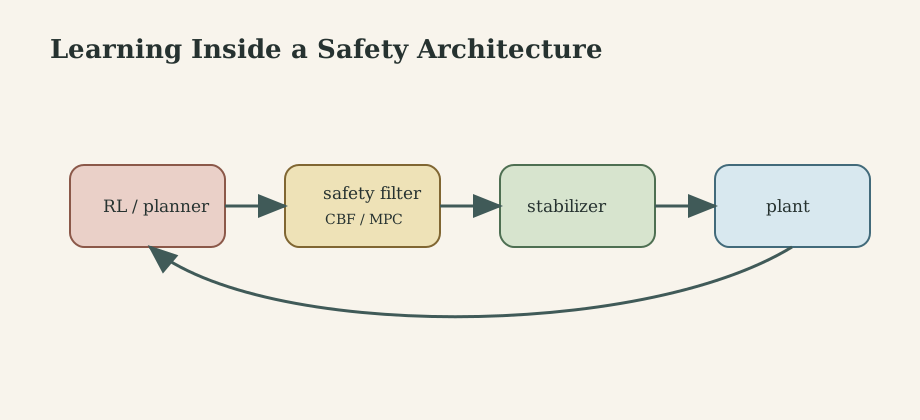
RL is strongest when simulation is abundant, models are incomplete, and long-horizon objectives matter. It is risky when exploration is unsafe, data are scarce, or worst-case guarantees dominate. In engineered control systems, learning should usually sit inside a safety architecture: robust baseline controller, MPC shield, Lyapunov or barrier filter, or backup policy.
What This Framework Lets Us Do
This framework helps choose among adaptation, optimization, robustness, and learning based on assumptions and required guarantees. The strongest systems often combine a safe inner loop, a predictive mid-level optimizer, and a learning or planning outer layer.
Where the Framework Stops Being Reliable
Theorems depend on matching conditions, smoothness, boundedness, excitation, noise models, and actuator assumptions. Sampling, saturation, delays, unmodeled dynamics, and unsafe exploration can break the clean proof story.
Where the Subject Leads Next
The next steps are adaptive backstepping, robust MPC, nonlinear $H_\infty$ control, control barrier functions, safe RL, Bayesian adaptive control, and learning-augmented model predictive control.
Technical and Editorial Audit
- Condensed the prior theorem-heavy note into a design map organized by guarantee type.
- Preserved internal links to the surrounding control notes.
- Added original figures for method selection, MRAC Lyapunov cancellation, robust modifications, optimal-control stack, and learning safety layers.
- Kept the central equations for MRAC, persistent excitation, PMP, HJB, LQR, robust control, and Bellman recursion.
- Marked attribution as personal synthesis because no source course code was present.
Main Sources Used in This Note
- P. A. Ioannou and J. Sun, Robust Adaptive Control.
- K. S. Narendra and A. M. Annaswamy, Stable Adaptive Systems.
- D. E. Kirk, Optimal Control Theory.
- H. K. Khalil, Nonlinear Systems.
- D. P. Bertsekas, Dynamic Programming and Optimal Control.