Control Theory Basics
This note is adapted from course materials for MNE3049 Control Principles at City University of Hong Kong. Instructor: course teaching staff.
Central Question
How can we use measured error and limited actuation to reshape a dynamical system so that it tracks, rejects disturbances, stays stable, and remains robust when the model is imperfect?
Control theory starts with a plant, not a gain. A heater stores thermal energy before its temperature changes. A motor-load system stores kinetic energy before speed changes. A robot joint may obey a commanded torque but still saturate, vibrate, delay, or amplify sensor noise. The controller is therefore not an add-on formula; it is a device for changing the closed-loop dynamics of an imperfect physical system.
The causal spine is:
\[\text{system boundary} \rightarrow \text{states, inputs, outputs, disturbances} \rightarrow \text{dynamic model} \rightarrow \text{open-loop behavior} \rightarrow \text{stability} \rightarrow \text{feedback} \rightarrow \text{time and frequency tradeoffs} \rightarrow \text{controller structure} \rightarrow \text{implementation limits}.\]If Signals & Systems gives the language of linear time-invariant models, control theory gives that language a purpose: shaping motion, regulation, and robustness under uncertainty.
1. Define the System Boundary First
A control problem begins by deciding what is inside the plant boundary and what is outside it.
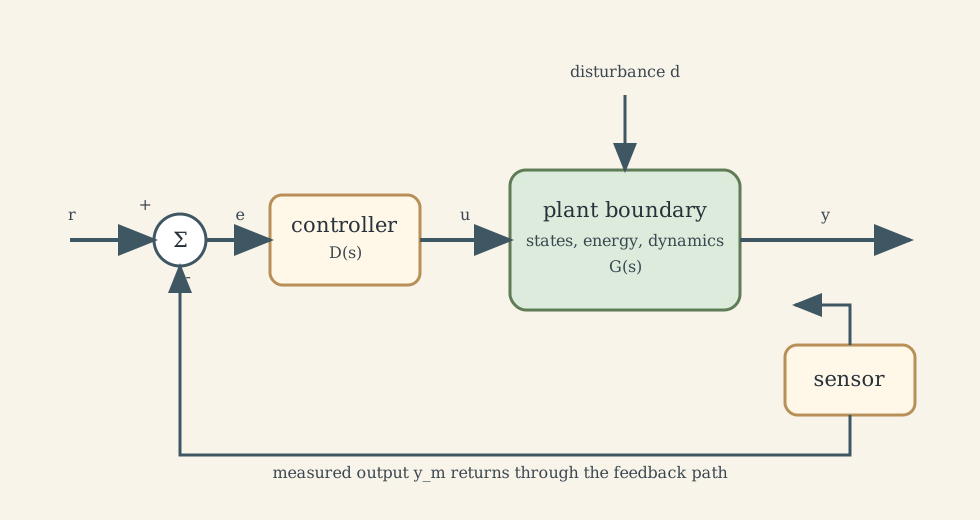
The usual roles are:
- plant: the physical or computational process we want to influence;
- input (u(t)): the actuator command we can choose;
- output (y(t)): the variable we care about regulating or tracking;
- reference (r(t)): the desired output;
- disturbance (d(t)): an external influence not commanded by the controller;
- measurement (y_m(t)): the sensor output actually available to the controller;
- controller (D): the algorithm that maps error and internal memory into (u).
This boundary matters because control is not “make the system do anything.” It is “use limited actuation and imperfect measurement to influence selected variables.” A controller cannot directly regulate an unmeasured variable unless it can infer it; it cannot move an unactuated mode unless the plant physics couples that mode to an input.
2. States, Parameters, and Operating Regimes
A state is the smallest set of variables that, together with future inputs, determines future behavior. For a heated chamber, temperature may be enough. For a mass-spring-damper, position and velocity are needed. For a circuit, capacitor voltages and inductor currents are natural states.
Parameters such as mass (m), damping (b), stiffness (k), thermal resistance (R), and thermal capacitance (C) are not states. They describe the plant. If they drift with temperature, wear, or payload, the model must either include that variation or treat it as uncertainty.
An operating point is a nominal condition around which we analyze behavior. Many plants are nonlinear, but local linear models can be accurate near a chosen operating regime. The model is valid only where its assumptions remain true:
- small deviations around the nominal point;
- actuator and sensor approximately linear;
- delays small relative to the controlled dynamics;
- unmodelled flexible modes far above the control bandwidth;
- parameters sufficiently constant over the design interval.
The assumptions are part of the model. They are not paperwork after the mathematics.
3. From Physics to Control Models
Two simple plants are enough to introduce most of classical control: a first-order thermal process and a second-order mechanical servo.
3.1 Thermal Process: One Dominant Stored-Energy State
Let (\theta(t)) be temperature rise above ambient. A simple energy balance gives
\[C\dot{\theta} = -\frac{1}{R}\theta + K_h u + d,\]where (C) is thermal capacitance ([\mathrm{J/K}]), (R) is thermal resistance ([\mathrm{K/W}]), (K_h u) is heater power ([\mathrm{W}]), and (d) is an unknown heat disturbance ([\mathrm{W}]).
With (\tau=RC), the model can be written as
\[\tau\dot{\theta}+\theta = K u + d_\theta.\]The physical meaning is direct: the chamber has one dominant memory state and one dominant time constant. If forcing stops, it forgets exponentially rather than instantly.
3.2 Mechanical Servo: Inertia, Dissipation, and Stiffness
For a mass-spring-damper driven by force,
\[m\ddot{x}+b\dot{x}+kx = u+d,\]where (m) is mass ([\mathrm{kg}]), (b) is damping ([\mathrm{N\,s/m}]), (k) is stiffness ([\mathrm{N/m}]), (u) is actuator force ([\mathrm{N}]), and (d) is disturbance force ([\mathrm{N}]).
This plant can overshoot and oscillate because it stores both kinetic and potential energy. The state-space form makes that memory explicit:
\[\dot{x}_1=x_2, \qquad \dot{x}_2=-\frac{k}{m}x_1-\frac{b}{m}x_2+\frac{1}{m}u+\frac{1}{m}d, \qquad y=x_1.\]In matrix form,
\[\dot{x}=Ax+Bu+Ed, \qquad y=Cx.\]3.3 Linearization
A nonlinear plant may be written as
\[\dot{x}=f(x,u,d), \qquad y=h(x,u,d).\]Around an equilibrium ((x_0,u_0,d_0)) satisfying (f(x_0,u_0,d_0)=0), small deviations satisfy
\[\delta\dot{x}=A\delta x+B\delta u+E\delta d, \qquad \delta y=C\delta x+D\delta u+F\delta d,\]where the matrices are Jacobians at the operating point. This is why classical control often works on nonlinear hardware: the loop is designed around the regime where the plant behaves approximately linearly.
4. Open-Loop Dynamics Before Control
Before adding feedback, ask how the plant moves by itself.
For the thermal plant with (u=d_\theta=0),
\[\theta(t)=\theta(0)e^{-t/\tau}.\]For a standard underdamped second-order mode,
\[x_n(t)=e^{-\zeta\omega_n t} \left(A\cos\omega_d t+B\sin\omega_d t\right), \qquad \omega_d=\omega_n\sqrt{1-\zeta^2}.\]Poles and eigenvalues summarize this natural motion:
- negative real poles give monotone decay;
- complex left-half-plane poles give decaying oscillation;
- poles near the imaginary axis settle slowly;
- right-half-plane poles grow and are unstable;
- imaginary-axis poles require special care because they do not decay.
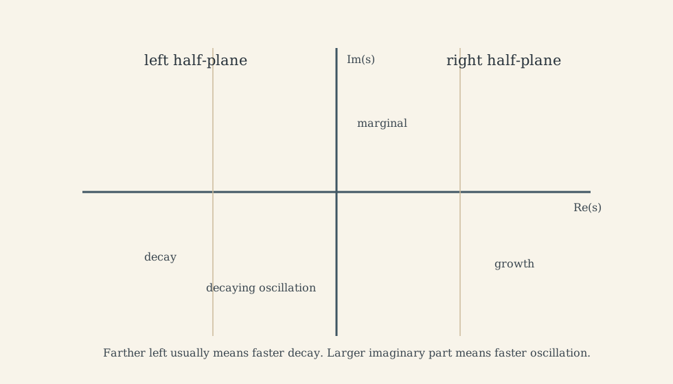
Control does not create dynamics from nothing. It moves or reshapes modes that already exist in the plant-controller interconnection.
5. Stability: Necessary but Not Sufficient
Stability is the first pass/fail test.
Internal stability asks whether internal states return or remain bounded after perturbation. BIBO stability asks whether bounded inputs produce bounded outputs. For minimal LTI systems these align closely, but they are conceptually different: hidden unstable modes can be dangerous even if a particular input-output transfer function hides them.
For continuous-time LTI systems, a common pole test is:
- all poles in the open left half-plane: asymptotically stable;
- repeated or uncontrolled imaginary-axis poles: marginal or unstable depending on structure;
- any right-half-plane pole: unstable.
Stability alone is not enough. A stable controller may still be too slow, too oscillatory, too noisy, too fragile, or impossible for the actuator to implement. The design problem is:
stabilize the plant with acceptable speed, damping, accuracy, noise sensitivity, saturation behavior, and robustness.
6. Transfer Functions and the Characteristic Equation
For an LTI model under zero initial conditions, the transfer function is
\[G(s)=\frac{Y(s)}{U(s)}.\]The zero-initial-condition phrase matters. A transfer function describes input-output behavior, not arbitrary stored initial energy.
For the running examples,
\[G_\theta(s)=\frac{\Theta(s)}{U(s)}=\frac{K}{\tau s+1}, \qquad G_x(s)=\frac{X(s)}{U(s)}=\frac{1}{ms^2+bs+k}.\]Poles are denominator roots and govern natural motion. Zeros are numerator roots and shape how inputs appear at the output. Non-minimum-phase zeros, delays, and hidden lightly damped modes can make control much harder.
For standard negative feedback with controller (D(s)), plant (G(s)), and sensor path (H(s)),
\[E(s)=R(s)-H(s)Y(s), \qquad U(s)=D(s)E(s), \qquad Y(s)=G(s)U(s).\]Thus,
\[\frac{Y(s)}{R(s)} = \frac{D(s)G(s)}{1+D(s)G(s)H(s)}.\]The characteristic equation is
\[1+D(s)G(s)H(s)=0.\]This is the core mathematical fact of feedback: the controller changes the denominator of the closed-loop system. It reshapes the poles, and therefore the motion.
7. Time-Domain Performance: Speed, Damping, Accuracy
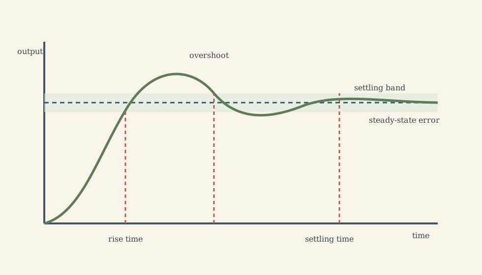
Step-response metrics are compact descriptions of transient and steady behavior:
- rise time: how quickly the output initially approaches the target;
- overshoot: how far the output exceeds the target;
- settling time: how long before it stays within a tolerance band;
- steady-state error: the final offset after transients die out.
The standard second-order closed-loop template is
\[G_{cl}(s)=\frac{\omega_n^2}{s^2+2\zeta\omega_n s+\omega_n^2}.\]For (0<\zeta<1),
\[M_p\approx e^{-\pi\zeta/\sqrt{1-\zeta^2}}\times 100\%, \qquad t_s\approx\frac{4}{\zeta\omega_n}\]for the common 2% settling-time approximation. These are design heuristics for dominant second-order behavior, not universal laws for every plant.
When the closed loop is stable, the final-value theorem gives
\[\lim_{t\to\infty}y(t)=\lim_{s\to 0}sY(s).\]Classical system type counts the number of open-loop integrators. More type improves polynomial tracking in ideal models, but integrators also add phase lag and can worsen robustness. Integral action is powerful because it removes constant steady-state error; it is dangerous because it adds controller memory that can wind up during saturation.
8. Frequency-Domain Design: Bandwidth, Margins, and Noise
Frequency response asks how the system reacts to sinusoidal inputs of different frequencies. For
\[G(s)=\frac{1}{\tau s+1},\]we evaluate (G(j\omega)):
\[|G(j\omega)|=\frac{1}{\sqrt{1+(\omega\tau)^2}}, \qquad \angle G(j\omega)=-\tan^{-1}(\omega\tau).\]A first-order plant follows slow commands well but attenuates and lags fast commands. That lag becomes dangerous when feedback tries to push bandwidth too high.
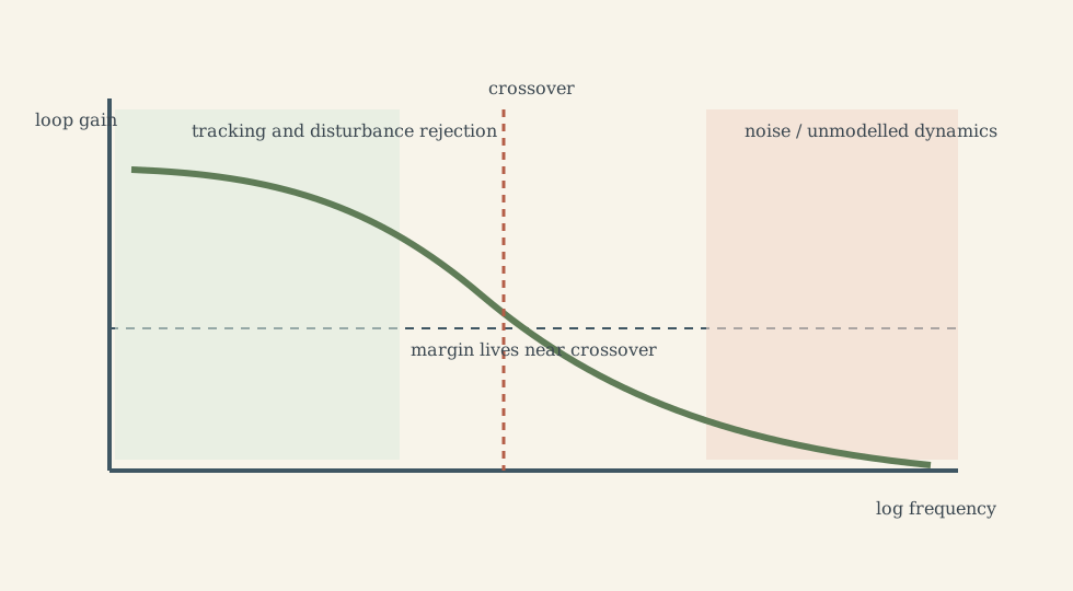
Important frequency-domain ideas:
- bandwidth estimates how fast the closed loop can respond;
- gain margin asks how much gain increase can be tolerated before instability;
- phase margin asks how much additional phase lag can be tolerated near crossover;
- Nyquist gives an exact closed-loop stability test from open-loop encirclements of (-1);
- Nichols combines gain and phase in a loop-shaping view.
These tools are not separate worlds. They are different projections of the same robustness problem.
9. Sensitivity and the Waterbed Tradeoff
Let the loop gain be
\[L(s)=D(s)G(s)H(s).\]The sensitivity and complementary sensitivity functions are
\[S(s)=\frac{1}{1+L(s)}, \qquad T(s)=\frac{L(s)}{1+L(s)}.\]They satisfy
\[S(s)+T(s)=1.\]Small (S) at low frequency means good tracking and disturbance rejection. Small (T) at high frequency means less sensor-noise transmission and less excitation of unmodelled fast dynamics. Since they sum to one, the controller cannot make both small everywhere. Control design is a redistribution of error, noise, and uncertainty across frequency.
This is the “waterbed” intuition: pushing sensitivity down in one region tends to push it up somewhere else, especially for plants with delays, right-half-plane zeros, or bandwidth limits.
10. Classical Design Views
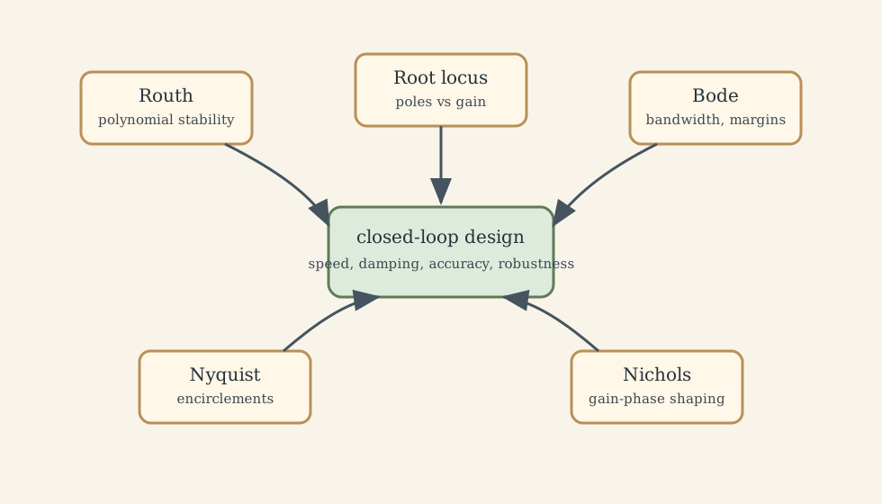
10.1 Routh-Hurwitz
Routh-Hurwitz checks whether a characteristic polynomial has right-half-plane roots without solving for all roots. For
\[s^3+a_2s^2+a_1s+a_0,\]a continuous-time cubic is stable if
\[a_2>0,\qquad a_1>0,\qquad a_0>0,\qquad a_2a_1>a_0.\]This is an algebraic sanity check for a controller-dependent denominator.
10.2 Root Locus
Root locus asks:
As a gain changes, where do the closed-loop poles move?
Branches start at open-loop poles and end at open-loop zeros or infinity. The plot makes visible whether increasing gain speeds the response, improves damping, or drives the loop unstable.
10.3 Bode, Nyquist, and Nichols
Bode plots expose bandwidth and margins. Nyquist connects open-loop frequency response to exact closed-loop stability. Nichols charts make loop-shaping tradeoffs visible in a gain-phase plane. They are complementary tools, not competing methods.
11. Controllers as Model-Shaping Tools
The standard PID form is
\[D(s)=K_P+\frac{K_I}{s}+K_Ds.\]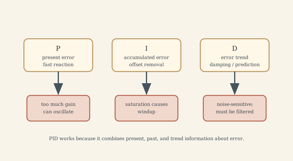
The terms have different physical meanings:
- P reacts to current error and tends to stiffen the response;
- I accumulates past error and can remove constant steady-state offset;
- D reacts to error trend and can add damping, but it is noise-sensitive.
Real derivative action is filtered; ideal differentiation is not implementable over infinite bandwidth. Real integral action needs anti-windup because actuators saturate. When saturation occurs, the actuator cannot realize the requested input, but the integrator may keep accumulating error. Anti-windup keeps controller memory consistent with actuator reality.
Lead and lag compensators express similar loop-shaping goals:
\[D_{lead}(s)=K\frac{1+\tau s}{1+\alpha\tau s},\qquad 0<\alpha<1,\] \[D_{lag}(s)=K\frac{1+\tau s}{1+\beta\tau s},\qquad \beta>1.\]Lead compensation adds phase near crossover and can improve damping or bandwidth. Lag compensation increases low-frequency gain while trying not to push crossover too high. Feedforward, reference shaping, and two-degree-of-freedom structures are added when tracking and disturbance rejection should not be forced through exactly the same path.
12. Implementation Limits: What Fails First
Control designs fail in hardware for reasons that may not appear in the first transfer function:
- actuator saturation and rate limits;
- sensor noise, quantization, bias, and delay;
- sampling and zero-order hold effects;
- unmodelled flexible modes;
- friction, backlash, dead zones, and stiction;
- parameter drift and payload variation;
- computational delay and numerical precision;
- unsafe transients during startup, shutdown, or fault recovery.
A practical validation workflow is:
- identify the plant boundary and safety limits;
- estimate or identify the model;
- design with margin rather than exact cancellation;
- simulate nominal, disturbed, saturated, and parameter-shifted cases;
- test at low gain and low authority first;
- log reference, measurement, input, saturation, and fault flags;
- increase bandwidth only after the limiting mechanism is understood.
Control is therefore both mathematics and commissioning discipline.
13. State-Space Bridge
Transfer functions are excellent for single-input/single-output loop design, but they hide internal structure. State-space models expose it:
\[\dot{x}=Ax+Bu, \qquad y=Cx+Du.\]The eigenvalues of (A) are internal modes. For minimal realizations, they correspond to transfer-function poles.
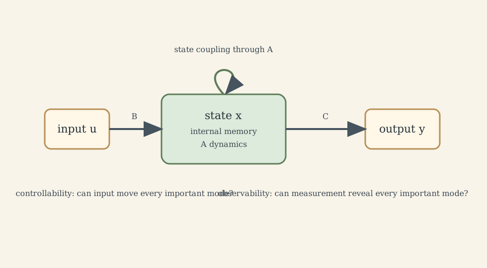
The controllability matrix is
\[\mathcal{C}=\begin{bmatrix}B & AB & \cdots & A^{n-1}B\end{bmatrix}.\]The observability matrix is
\[\mathcal{O}= \begin{bmatrix} C\\ CA\\ \vdots\\ CA^{n-1} \end{bmatrix}.\]Full rank means every mode can be influenced or seen through the chosen channels. No controller can move a mode it cannot actuate; no observer can reconstruct a mode that leaves no measurement signature.
With full-state feedback,
\[u=-Kx+Nr, \qquad A_{cl}=A-BK.\]This is the modern version of the same idea: choose feedback to move closed-loop modes.
For the full multivariable story, continue to Modern, Multivariable, and Networked Control.
14. Bridge to Nonlinear Control
Classical control is usually local. It assumes the model is approximately linear near the operating point and that the plant stays in the region where the design assumptions hold.
Real plants may include saturation, switching, friction, impacts, geometric nonlinearities, dead zones, gain scheduling, and constraints. Linear tools still help locally, but global behavior needs phase-plane reasoning, Lyapunov analysis, invariant sets, nonlinear compensation, or hybrid analysis.
For those topics, continue to Topics in Nonlinear Systems. For adaptive, optimal, robust, and learning-based extensions, continue to Adaptive, Optimal, Robust, and Learning Control.
What This Framework Lets Us Do
This framework lets us reason through control as an engineering workflow:
- choose a system boundary;
- identify states, inputs, outputs, disturbances, and measurements;
- derive or identify a model;
- inspect natural dynamics and stability;
- close the loop to reshape the characteristic equation;
- trade speed, damping, steady-state error, noise, saturation, and robustness;
- validate on the real system without trusting the nominal model too much.
Where the Framework Stops Being Reliable
The framework becomes unreliable when its assumptions are violated: large nonlinear excursions, strong delays, saturating actuators, hidden flexible modes, changing parameters, poor sensing, unmodelled constraints, or unsafe test conditions. In those regimes, the local LTI design may still be a useful inner loop, but it must be checked with nonlinear, robust, sampled-data, or experimental methods.
Where the Subject Leads Next
Basic control leads naturally to:
- state-space control and observers;
- multivariable and networked control;
- nonlinear stability and Lyapunov methods;
- robust and (H_\infty) loop shaping;
- optimal control and MPC;
- adaptive and learning-based control;
- mechatronic implementation, where sensors, actuators, computation, and safety limits decide what the math can actually achieve.
Compact Recall Map
- Control starts by defining the plant boundary.
- A useful model names states, inputs, outputs, disturbances, and assumptions.
- Open-loop poles describe the plant’s natural motion.
- Feedback changes the characteristic equation and reshapes closed-loop poles.
- Stability is necessary but not enough.
- Time-domain tools describe speed, damping, and accuracy.
- Frequency-domain tools describe bandwidth, margins, noise, and robustness.
- PID, lead, lag, feedforward, and 2-DOF designs are loop-shaping tools.
- State-space methods expose controllability, observability, and internal modes.
- Nonlinear and implementation limits decide where the basic model stops being safe.
Technical and Editorial Audit
| Area | Correction or decision |
|---|---|
| Central question | Reframed basic control around limited actuation, measurement, stability, robustness, and implementation. |
| Preserved material | Retained thermal and mass-spring-damper examples, transfer functions, second-order metrics, Routh-Hurwitz cubic condition, sensitivity functions, PID/lead/lag, and internal links. |
| Units | Added units for the thermal and mechanical model variables and parameters. |
| Assumptions | Made linearization, zero initial conditions, dominant second-order formulas, and local LTI validity explicit. |
| Sign conventions | Used standard negative feedback with (e=r-y_m) and characteristic equation (1+DGH=0). |
| Figures | Added seven original SVG diagrams for loop boundary, pole geometry, step metrics, Bode tradeoff, classical design views, PID terms, and state-space structure. |
| Safety | Added implementation limits and a cautious validation workflow before increasing controller authority. |
| Internal links | Preserved links to Signals & Systems, Modern Control, Nonlinear Systems, and Adaptive/Optimal/Robust/Learning Control. |
Sources and Further Reading
- CityU MNE3049 course material.
- K. Ogata, Modern Control Engineering.
- G. F. Franklin, J. D. Powell, and A. Emami-Naeini, Feedback Control of Dynamic Systems.
- K. J. Astrom and R. M. Murray, Feedback Systems, freely available at https://fbsbook.org/.