Modern, Multivariable, and Networked Control
This note is adapted from course materials for FEL3210 Multivariable Control and FEL3330 Networked and Multi-Agent Control Systems at KTH Royal Institute of Technology. Instructors: course teaching staff.
Central Question
Modern control asks a different question from classical loop shaping: what internal state, information pattern, and uncertainty model are needed to make a coupled dynamic system behave well?
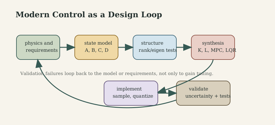
Classical design often begins with one transfer function and one loop. Modern control begins with a state model:
\[\dot x = Ax + Bu, \qquad y = Cx + Du.\]This representation keeps internal modes visible. It also scales naturally to sampled controllers, MIMO plants, observers, optimal control, robust design, and networked agents.
1. State-Space Models
The state $x(t)$ is the information needed, together with future inputs, to predict future behavior. In an LTI model:
- $A$ encodes free dynamics and natural modes,
- $B$ encodes actuator authority,
- $C$ encodes what sensors reveal,
- $D$ encodes direct input-output feedthrough.
For a mass-spring-damper system
\[m\ddot q + b\dot q + kq = u,\]choosing $x_1=q$, $x_2=\dot q$ gives
\[\dot x = \begin{bmatrix} 0 & 1 \\ -k/m & -b/m \end{bmatrix}x+ \begin{bmatrix} 0 \\ 1/m \end{bmatrix}u.\]The point is not only algebraic neatness. The state model tells us which physical energy-storage modes exist, how they are coupled, and which ones can be actuated or measured.
2. Structural Tests: Can We Control and Observe It?
For $\dot x=Ax$, stability follows from eigenvalues of $A$: continuous-time asymptotic stability requires all eigenvalues in the open left-half plane.
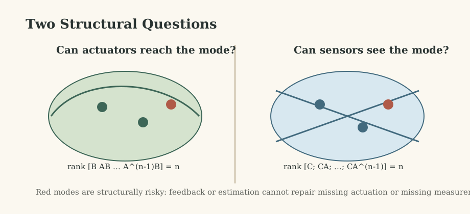
Controllability asks whether inputs can move every state direction:
\[\mathcal{C}=\begin{bmatrix}B & AB & A^2B & \cdots & A^{n-1}B\end{bmatrix}, \qquad \operatorname{rank}\mathcal{C}=n.\]Observability asks whether outputs reveal every internal mode:
\[\mathcal{O}= \begin{bmatrix} C\\ CA\\ \vdots\\ CA^{n-1} \end{bmatrix}, \qquad \operatorname{rank}\mathcal{O}=n.\]These are design gates. If an unstable mode is uncontrollable, feedback cannot move it. If an important mode is unobservable, an observer cannot reconstruct it from the available measurements.
3. Feedback, Observers, and Separation
Full-state feedback uses
\[u=-Kx+Nr,\]which yields closed-loop dynamics
\[\dot x=(A-BK)x+BNr.\]If $(A,B)$ is controllable, the closed-loop poles can be assigned through $K$. In practice, pole placement is most useful for intuition and small systems; for larger coupled systems, optimal or robust methods often give better-conditioned designs.
When $x$ is not measured directly, a Luenberger observer estimates it:
\[\dot{\hat x}=A\hat x+Bu+L(y-C\hat x).\]The estimation error $\tilde x=x-\hat x$ follows
\[\dot{\tilde x}=(A-LC)\tilde x.\]For LTI systems, the separation principle says controller poles and observer poles can be designed independently when controllability and observability hold. The practical caveat is important: noise, delay, saturation, and model error still couple the designs in implementation.
4. MIMO Control Is Not Many Independent SISO Loops
For a multivariable plant,
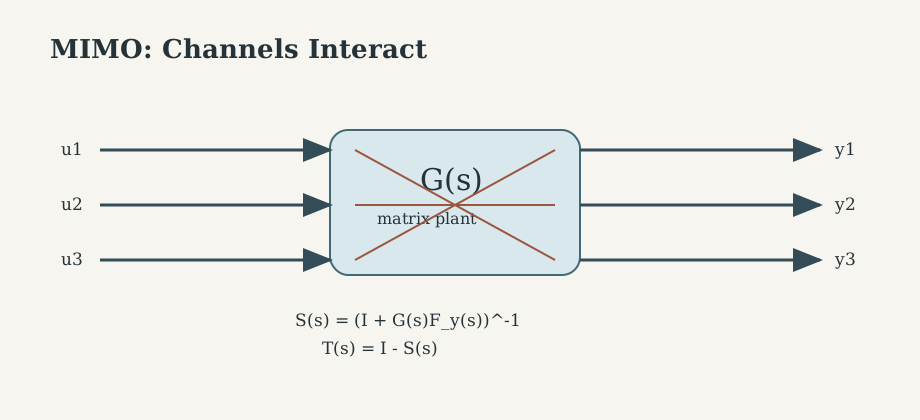
\[Y(s)=G(s)U(s),\]the entries of $G(s)$ reveal interaction: one actuator can influence several outputs, and one output may need several actuators. Pairing, decoupling, and robustness are therefore structural decisions, not tuning afterthoughts.
The sensitivity functions generalize to matrices:
\[S(s)=\left(I+G(s)F_y(s)\right)^{-1}, \qquad T(s)=I-S(s).\]Good multivariable design balances disturbance rejection, actuator effort, channel interaction, and uncertainty. If decentralized loops are used, the reason should be justified by weak coupling, robust pairing, or implementation constraints rather than convenience.
5. Optimal and Predictive Control
Linear Quadratic Regulator design chooses $u=-Kx$ to minimize
\[J=\int_0^\infty (x^\top Qx+u^\top Ru)\,dt.\]The matrices $Q$ and $R$ encode a design philosophy: which state deviations are expensive, and how costly actuator effort should be. The gain is obtained from an algebraic Riccati equation.
LQG combines LQR with a Kalman filter. The controller handles optimal regulation, while the estimator handles noisy measurements under linear-Gaussian assumptions.
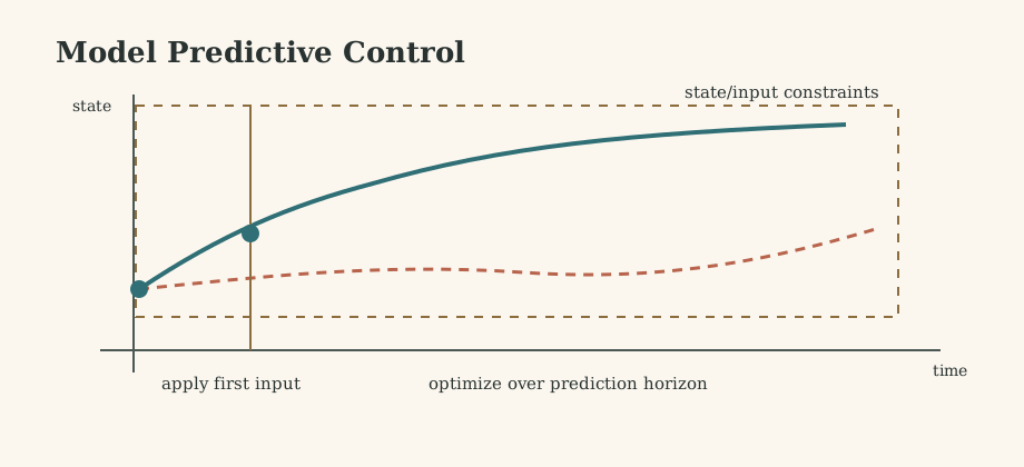
Model Predictive Control repeatedly solves a constrained finite-horizon problem:
- predict future state trajectories,
- optimize inputs subject to constraints,
- apply the first input,
- measure again and repeat.
MPC is especially natural for MIMO plants because input bounds, state limits, and coupled dynamics are part of the optimization problem rather than external patches.
6. Robustness, Sampling, and Implementation
Real controllers run on imperfect models and processors. A continuous controller becomes software or firmware with a sampling period, quantization, computation delay, actuator saturation, and sensor noise.
In discrete time,
\[x_{k+1}=A_d x_k+B_d u_k,\qquad y_k=C_d x_k+D_d u_k,\]stability moves from the left-half $s$-plane to the inside of the unit circle in the $z$-plane. Sampling should be chosen from bandwidth, delay margin, sensor noise, and actuator limits, not by a generic rule alone.
Robust control formalizes uncertainty. $H_\infty$ design minimizes worst-case amplification from disturbances to performance outputs, while structured singular value ideas track block-structured uncertainty. The engineering lesson is broader than any one method: state what model errors are protected against, and validate performance over that model family.
7. Networked and Multi-Agent Control
For single-integrator agents
\[\dot x_i=u_i,\]a basic consensus controller is
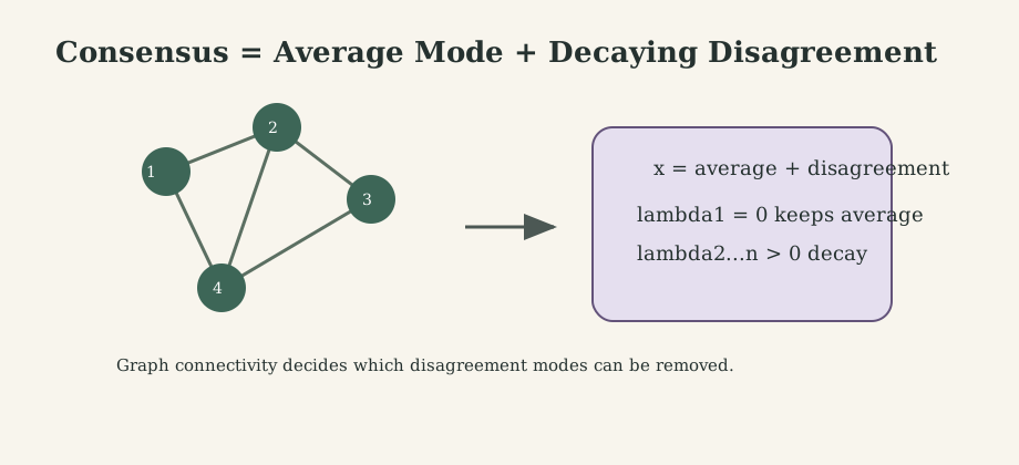
\[u_i=-\sum_{j\in\mathcal{N}_i}a_{ij}(x_i-x_j).\]Stacking all states gives
\[\dot x=-(L\otimes I)x,\]where $L$ is the graph Laplacian. For a connected undirected graph, $L$ is positive semidefinite and has one zero eigenvalue corresponding to the consensus direction. All disagreement modes decay, so agents converge to a common value.
Leader-follower tracking, formation control, distributed estimation, and cooperative MPC extend this logic by changing the graph, objectives, constraints, or information pattern.
What This Framework Lets Us Do
Modern control lets us design systems where internal state, coupling, constraints, uncertainty, and network structure matter simultaneously. It is the natural bridge from classical feedback to robotics, power systems, process control, autonomous vehicles, and distributed infrastructure.
Where the Framework Stops Being Reliable
Linear models are local approximations. If saturation, contact, switching, delays, unmodeled resonances, packet loss, or human interaction dominate behavior, state-space methods still help, but the design must be extended with nonlinear analysis, hybrid models, robust validation, or experiments.
Where the Subject Leads Next
For loop shaping, root locus, Nyquist, and classical compensators, see Control Theory Basics. For Lyapunov geometry, backstepping, sliding mode, and nonlinear design, see Topics in Nonlinear Systems. For adaptive, optimal, robust, and learning guarantees, see Adaptive, Optimal, Robust, and Learning Control.
Technical and Editorial Audit
- Corrected the emphasis from a list of methods to the causal design chain: model, structural tests, synthesis, robustness, implementation.
- Kept the course attribution in the main body rather than front matter.
- Preserved internal links to the surrounding control-note sequence.
- Added original figures for state-space workflow, structural tests, MIMO sensitivity, MPC, and consensus modes.
- Claims are standard LTI/control facts; exact controller synthesis details require numerical plant data and software verification.
Main Sources Used in This Note
- K. J. Astrom and R. M. Murray, Feedback Systems.
- T. Kailath, Linear Systems.
- S. Skogestad and I. Postlethwaite, Multivariable Feedback Control.
- D. P. Bertsekas, Dynamic Programming and Optimal Control.
- R. Olfati-Saber, J. A. Fax, and R. M. Murray, “Consensus and Cooperation in Networked Multi-Agent Systems.”